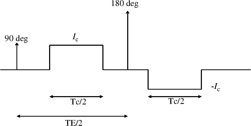
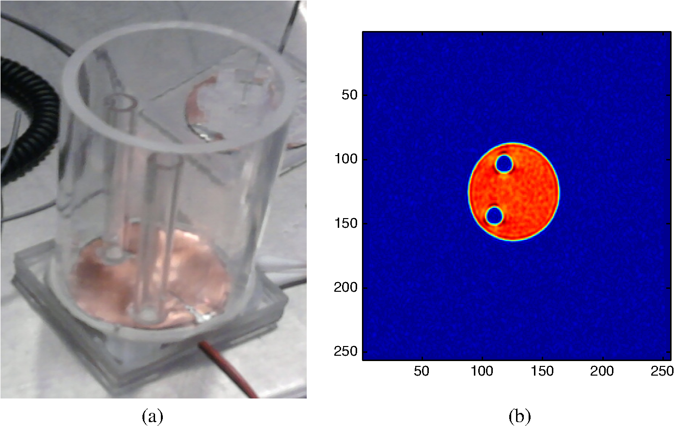
1.

Introduction

Low frequency current density imaging (LFCDI) is a magnetic resonance imaging (MRI)-based technique which measures current density inside a subject while a current pulse is injected into the subject. The method was developed in the late 1980s and early 1990s by Joy et al.^1,2 This method has been tested on phantoms^1,3,4 and also applied to the in vivo and ex vivo tissues in order to obtain the current density map inside the subject.^5–9 The method works based on the fact that the magnetic flux induced by injected current can be measured using phase changes recorded in MRI phase images.¹ Although it is a very useful method to study the current density maps, like any other method it has some limitations in terms of image quality and implementation. The images can become very noisy and unusable if acquisition parameters are not chosen appropriately, the energy of the injected current pulse is not enough, or the size of the studied subject is very small. The noise and its effect on the current density images are studied in the literature in two main works by Scott et al.¹⁰ and Sadlier et al.¹¹ The former studied the effect of MRI acquisition parameters like echo time (TE), injected current pulse width (Tc), and current amplitude on the noise level in the images. The latter used the fact that the noise distribution in real and imaginary images is zero mean Gaussian. These real and imaginary images are used to calculate the phase changes generated by induced magnetic flux. Sadlier et al. subsequently studied the effect of this Gaussian noise on the magnetic flux induced in one direction and also investigated the effect of the strength of the main magnetic field of the MRI machine on the level of measurable currents. Another work by Lee et al.¹² suggested ramp-preserving denoising for CDI images by developing a new ramp preserving method based on the Perona–Malik denoising method.¹³

In this work, the probability distribution of the measured phase for each pixel inside the subject is derived and the current density distribution is approximated. Furthermore, because the distribution of noise in the real and imaginary images is Gaussian and in the current density case the derived distribution will be shown to be close to a Gaussian, three different denoising methods are applied on a cylindrical phantom. These three methods are ramp-preserving Perona–Malik (PM) denoising,¹³ two-dimensional adaptive Wiener filter,¹⁴ and the state-of-the-art block-matching and three-dimensional (BM3D) filtering.¹⁵ The PM method is chosen as a ramp-preserving method already used for CDI images, Wiener as a smoothing method, and BM3D because it is shown to have a better performance compared with the traditional denoising methods.¹⁵ The denoising is performed at two different stages: first on the initial noisy real and imaginary images recorded by MRI machine and second on the final current density maps, and the results are compared with the desired noiseless current density maps.

2.

Method

The experimental data used in this paper were obtained by performing a CDI experiment on a cylindrical phantom filled with $9\mathrm{g}/\mathrm{L}·\mathrm{NaCl}$ and $0.64\mathrm{g}/\mathrm{L}·{\mathrm{CuSO}}_4$ solution with $T2=170\mathrm{ms}$ and $T1=200\mathrm{ms}$.¹⁶ The phantom had a diameter of 4.5 cm and length of 9 cm. Two datasets were obtained: for set 1, the current amplitude was 20 mA and for set 2 the current was 45 mA. The first dataset had six slices and the second one had five slices. The current pulses were generated by a pulse generator circuit and amplified using an HP Harrison 6824A power supply-amplifier which supports maximum peak-to-peak voltage of 50 V for currents up to 1 A. The current injection system was constant current source. The current was maintained constant and was measured as a voltage across a $10\mathrm{\Omega }$ resistor in series with the phantom. Imaging was conducted in a 1.5 T GE machine at Toronto General Hospital. The acquisition parameters were TE equal to 40 ms, Tc equal to 18 ms, number of excitations equal to 2, repetition time equal to 700 ms, a field of view of 15 cm, and the image size was $256\times 256$ pixels. The current was injected through copper disc electrodes at the top and bottom of phantom. The current pulse sequence for LFCDI is shown in Fig. 1.¹⁷

Fig. 1

Low frequency current density imaging (LFCDI) current pulse sequence for one phase cycle.

The axis of the cylinder was aligned with the $z$-direction and it was parallel to the direction of the current. The coordinate system was adopted from Scott et al.¹⁷ in which the $z$-direction is perpendicular to the main magnetic field. The slices were equally spaced and were perpendicular to the $z$-axis. Two hollow bars of Plexiglas were positioned inside the phantom to track different orientations. Due to the symmetry of the cylinder, there was only one component of current density, which was in the $z$-direction. Therefore, only Bx and By were measured by having a 90-deg rotation of the cylinder around its axis. A spin-echo sequence was used for imaging and six slices were defined with equivalent distance and in the $x-y$ plane. Figure 2 shows the empty phantom used for this experiment and the magnitude image for one slice.

Fig. 2

(a) The cylindrical phantom, and (b) magnitude image for one slice.

2.1.

Distribution of Noise

As reported in the literature, the noise in the background of real and imaginary images is zero mean Gaussian.¹¹ This fact was experimentally verified for the phantom experiment. The histograms of background for real and imaginary images in a slice are shown in Figs. 3(a) and 3(b), respectively, with a Gaussian distribution fitted to the samples (solid curve). The Gaussian distribution fitted to Fig. 3 has standard deviations of 10.75 and 10.57 for Figs. 3(a) and 3(b), respectively, and means of $-0.04$ and $-0.08$ for Figs. 3(a) and 3(b), respectively. It can be seen that the distribution of background noise is almost zero mean Gaussian and it has approximately the same distribution for real and imaginary images. The standard deviation of this noise can be extracted from the background.^11,18 Therefore, if we assume that for each pixel inside the subject $X_R$ is the random variable representing the corrupted intensity in real images and $X_I$ is the random variable representing the corrupted intensity in imaginary images, we have for one pixel

Eq. (1)

$$X_R=R+N_R\hspace{1em}{N}_R\sim N(0,\sigma ),$$

Eq. (2)

$$X_I=I+N_I\hspace{1em}{N}_I\sim N(0,\sigma ).$$

Fig. 3

(a) Histogram of background noise in real image of a slice, and (b) histogram of background noise in imaginary image of the same slice.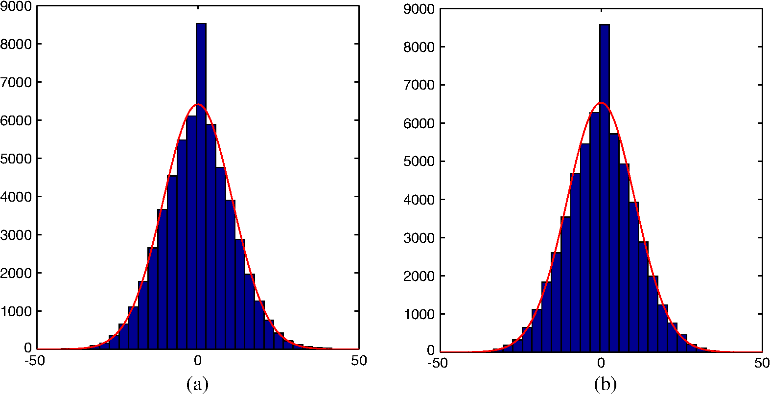

$N_R$ is the noise random variable for the chosen pixel in the real image and $N_I$ is the random variable representing noise in the imaginary image for the same pixel. Therefore, $X_R$ and $X_I$ are Gaussian at each pixel with nonzero means $R$ and $I$ at that pixel. In this case, the joint distribution of $X_R$ and $X_I$ is a bivariate Gaussian distribution given as

Eq. (3)

$$f(X_R,X_I)=\frac{1}{\pi {\nu }^2}\exp (-[\frac{{(X_R-R)}^2}{{\nu }^2}+\frac{{(X_I-I)}^2}{{\nu }^2}\left]\right)\mathrm{while}\nu =\sqrt{2}\sigma .$$

The distribution of the angle and magnitude of $X_R+i{X}_I$ can be found using the Jacobian of the transformation as

Eq. (4)

$$f(\theta ,r)=\frac{1}{\pi {\nu }^2}r·\exp (-[\frac{(I^2+R^2+r^2-2rI\sin (\theta )}{{\nu }^2}-\frac{2rR\cos (\theta )}{{\nu }^2}\left]\right)\mathrm{while}\theta =\arg (X_R+i{X}_I)\mathrm{and}r=\sqrt{X_R^2+X_I^2}.$$

The symbol arg represents the argument of ($X_R+i{X}_I$). Because the current density is measured from the phase changes, we find $f(\theta )$ by integrating over $r$

Eq. (5)

$$f(\theta )=\frac{1}{\pi {\nu }^2}{\int }_0^{\infty }r·\exp (-[\frac{(I^2+R^2+r^2-2rI\sin (\theta )}{{\nu }^2}-\frac{2rR\cos (\theta )}{{\nu }^2}\left]\right)\mathrm{d}r=\frac{e^{-\frac{(I^2+R^2)}{{\nu }^2}}}{\pi {\nu }^2}{\int }_0^{\infty }r·\exp (-[\frac{(r^2-2rI\sin (\theta )}{{\nu }^2}-\frac{2rR\cos (\theta )}{{\nu }^2}\left]\right)\mathrm{d}r.$$

Defining

Eq. (6)

$$C=2I\cos (\theta )+2R\sin (\theta ),$$

Eq. (7)

$$=\frac{e^{-\frac{(I^2+R^2)}{{\nu }^2}}}{\pi {\nu }^2}{\int }_0^{\infty }r·\exp (-[\frac{{(r-\frac{C}{2})}^2-\frac{C^2}{4}}{{\nu }^2}\left]\right)\mathrm{d}r,$$

Eq. (8)

$$=\frac{e^{-\frac{(I^2+R^2)}{{\nu }^2}}{e}^{\frac{C^2}{4{\nu }^2}}}{\pi {\nu }^2}{\int }_0^{\infty }r·\exp (-[\frac{{(r-\frac{C}{2})}^2}{{\nu }^2}\left]\right)\mathrm{d}r.$$

Changing variable $u=r-(C/2)$,

Eq. (9)

$$=\frac{e^{-\frac{(I^2+R^2)}{{\nu }^2}}{e}^{\frac{C^2}{4{\nu }^2}}}{\pi {\nu }^2}({\int }_{-\frac{C}{2}}^{\infty }u·\exp (-\left[\frac{u^2}{{\nu }^2}\right])\mathrm{d}u+{\int }_{-\frac{C}{2}}^{\infty }\frac{C}{2}·\exp (-[\frac{u^2}{{\nu }^2}\left]\right)d\mathrm{u}).$$

Using the following identities

Eq. (10)

$$\int e^{-a{x}^2}\mathrm{d}x=\frac{\sqrt{\pi }}{2\sqrt{a}}=\mathrm{erf}(x\sqrt{a})a>0,$$

Eq. (11)

$$\int x{e}^{-a{x}^2}\mathrm{d}x=-\frac{1}{2a}{e}^{-a{x}^2},$$

the distribution can be simplified to

Eq. (12)

$$f(\theta )=\frac{e^{-\frac{(I^2+R^2)}{{\nu }^2}}}{\pi {\nu }^2}\{\frac{{\nu }^2}{2}+\frac{C\nu \sqrt{\pi }}{4}{e}^{\frac{C^2}{4{\nu }^2}}[1-\mathrm{erf}(-\frac{C}{2\sqrt{\nu }})]\}\mathrm{while}-\pi \le \theta \le \pi .$$

While erf is Gaussian error function, Eq. (12) shows the wrapped phase distribution. Unwrapping will not change the distribution, it will only shift the mean by $2k\pi$. The unwrapped values are proportional to the induced magnetic flux ($B$). Therefore, we can reason that $B$ at each point has a distribution similar to Eq. (12) just scaled or shifted.

To calculate each component of current density, derivatives of two perpendicular components of the induced $B$ should be used. The derivatives are calculated using derivative templates.¹⁰ These derivative templates rely on an averaging operation in a neighborhood to approximate the derivatives, therefore, their application compromises the spatial resolution and itself acts like denoising. If a $3\times 3$ template is used, the nine values of $Bs$ in the neighborhood of each point are used to calculate the derivative at each point and two derivatives. Therefore, the final distribution is the summation of 18 scaled distributions of the form provided in Eq. (12). Using the fact that the distribution of summation is a convolution of the distributions, we can find the final distribution of the current density ($J$). It is also known that the convolution of Gaussians is Gaussian,¹⁹ therefore, if the distribution in Eq. (12) is close to Gaussian, we can conclude the noise distribution in the measured current density is also Gaussian. Figures 4 and 5 show the distribution for various values of $R$, $I$, and $\sigma$. The values chosen for $R$ and $I$ in these figures are arbitrarily chosen in the range of observed values for real and imaginary images. These figures show the mean is dependent on $R$ and $I$_, while the variance depends on $R$, $I$, and $\sigma$. We can also conclude that the distribution in Eq. (12) can be approximated by a Gaussian for each point. The Gaussian claim for $f(\theta )$ can be quantified using kurtosis and skewness measures.²⁰ Furthermore, the normality of distribution based on its samples can be classified using the D’Agostino test²⁰ which is based on kurtosis and skewness. The results for Figs. 4 and 5 are shown in Table 1. The significance level used for the D’Agostino test in this table is 0.01. The table shows that for all the cases investigated in Figs. 4 and 5 except for one case, the distributions can be safely approximated by a Gaussian. However in order to find the ranges of $R$, $I$, and $\sigma$ for which the Gaussian approximation holds, the kurtosis, skewness, and D'Agostino test results for various ranges of $R$ and $I$ (between 1 and 100 with step of 5) and $\sigma$ are shown in Fig. 6. The significance level used for the D’Agostino test is 0.01. It can be seen that the ratio of magnitude $\sqrt{R^2+I^2}$ to $\sigma$ determines whether the Gaussian assumption holds. As this ratio increases, the distribution gets closer to a Gaussian. In both of our datasets, this ratio is close to 50 for a $\sigma$ of approximately 10, which means the distribution at each point can be approximated by a Gaussian. We can verify the distribution of noise in the phantom by performing a baseline analysis.²¹ In this case, we record real and imaginary images twice when there is no current in each orientation. The current is then calculated by considering repeated images in each orientation as two phase cycles of the CDI method.²¹ The resulting current density map in $\mathrm{A}/{\mathrm{m}}^2$ and its histogram are shown in Figs. 7(a) and 7(b). This histogram is reflective of the noise distribution because there is not much change in real and imaginary images in the absence of injected current, thus the real and imaginary images should be almost constant. Figures 7(c) and 7(d) and 7(e) and 7(f) show the calculated current density maps and their histograms when current is injected for Dataset 1 and Dataset 2, respectively. It can be seen that the noise distribution is only shifted when the current is injected. The red curves on the histograms show the Gaussian distributions fitted on the samples. For the no current case, the mean of the fitted Gaussian is 0.03 and its standard deviation is 3.62. The Gaussian fitted for Dataset 1 has mean of 13.24 and standard deviation of 3.67, while for Dataset 2 the Gaussian has mean of 29.45 and standard deviation of 3.19. This matches the fact that the convolution of 18 Gaussians (for the case of a $3\times 3$ derivative template) is Gaussian itself and, therefore, the final $J$ has a noise which is Gaussian while its mean and variance depend on the $R$, $I$, and noise in the real and imaginary images. In all three cases in Fig. 7, the background noise has almost the same zero mean Gaussian distribution with a standard deviation of approximately 10 and the noise in the current density images is also zero mean Gaussian with a standard deviation around 3. For the cases where a current was injected, $R$ and $I$ are not constant because of phase changes induced by the current. However, the magnitude $\sqrt{R^2+I^2}$ is constant for all three cases in Fig. 7 because the phantom has the same homogeneous structure. Looking back at Eq. (12), we can see that if the background noise $\sigma$ is constant and the magnitude $\sqrt{R^2+I^2}$ is constant, then the distribution $f(\theta )$ only depends on $C$. Functions $C$ in Eq. (6) for various $R$s and $I$s satisfying a constant $R^2+I^2$ are the same; they are only shifted. This can be shown mathematically as

Eq. (13)

$$R\cos (\theta +\varphi )+I\sin (\theta +\varphi )=R^{\prime }\cos (\theta )+I^{\prime }\sin (\theta ),$$

where $R^{\prime }=R\cos (\varphi )+I\sin (\varphi )$, $I^{\prime }=I\cos (\varphi )-R\sin (\varphi )$, and $R^{\prime 2}+I^{\prime 2}=R^2+I^2$. This can also be verified by plotting $f(\theta )$ for a constant $R^2+I^2$ which is shown in Fig. 8.

Fig. 4

(a) Probability distribution of $\theta$ [Eq. (12)], shown for pixels with various noiseless imaginary values, noiseless real value of 15 ($R=15$), and standard deviation of noise $\sigma =15$. (b) The probability distribution of $\theta$ [Eq. (12)] for a pixel with various noise levels, noiseless real value of 70 ($R=70$), and noiseless imaginary value of 50 (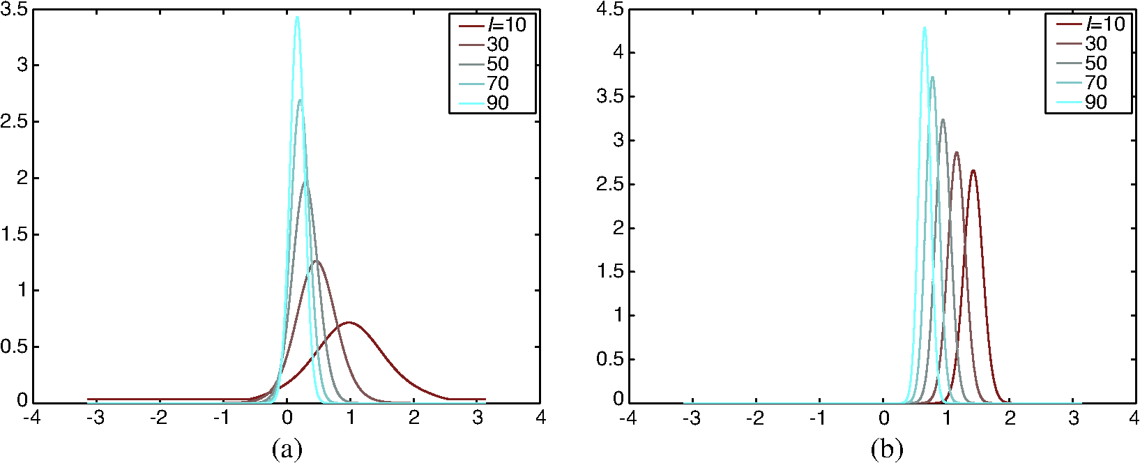$I=50$).

Fig. 5

(a) Probability distribution of $\theta$ [Eq. (12)], shown for pixels with various background noise standard deviations for $R=70$ and $I=50$. (b) The distribution in (a) zoomed for $\theta$ between 0 and 2 rad.

Table 1

Kurtosis, skewness, and D’Agostino test results for Figs. 4 and 5.

R	I	σ	Kurtosis	Skewness	D'Agostino test
70	50	4	2.9216	$-0.0016$	Normal
70	50	8	2.8912	$-0.0018$	Normal
70	50	12	2.8632	$-7.1852\times {10}^{-4}$	Normal
70	50	16	2.8496	$-4.0417\times {10}^{-4}$	Normal
70	50	20	2.8464	$-0.0013$	Normal
70	50	24	2.8384	−6.5718 × 10−4	Normal
15	10	15	2.7142	$3.6240\times {10}^{-4}$	Non-normal
15	30	15	2.8493	$-5.4670\times {10}^{-4}$	Normal
15	50	15	2.8418	$1.1330\times {10}^{-14}$	Normal
15	70	15	2.8530	$-4.4175\times {10}^{-4}$	Normal
15	90	15	2.8598	$-6.9692\times {10}^{-4}$	Normal
70	10	15	2.8513	$-0.0021$	Normal
70	30	15	2.8493	0.0017	Normal
70	50	15	2.8587	$7.0504\times {10}^{-4}$	Normal
70	70	15	2.8702	$2.5749\times {10}^{-4}$	Normal
70	90	15	2.8707	0.0011	Normal

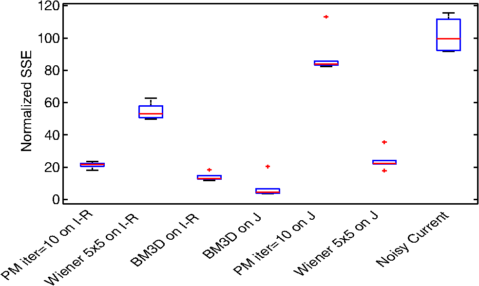
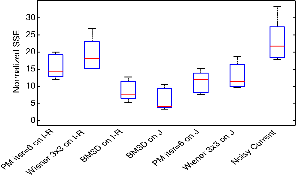
Fig. 6

(a), (d), and (g) kurtosis map of distribution $f(\theta )$ for various $R$s and $I$s for $\sigma$ equal to 8, 16, and 24, respectively. (b), (e), and (h) Skewness map of distributions for various $R$s and $I$s for $\sigma$ equal to 8, 16, and 24, respectively. (c), (f), and (i) D’Agostino test results for the distributions for various $R$s and $I$s for $\sigma$ equal to 8, 16, and 24, respectively, while dark red means Gaussian and dark blue means non-Gaussian.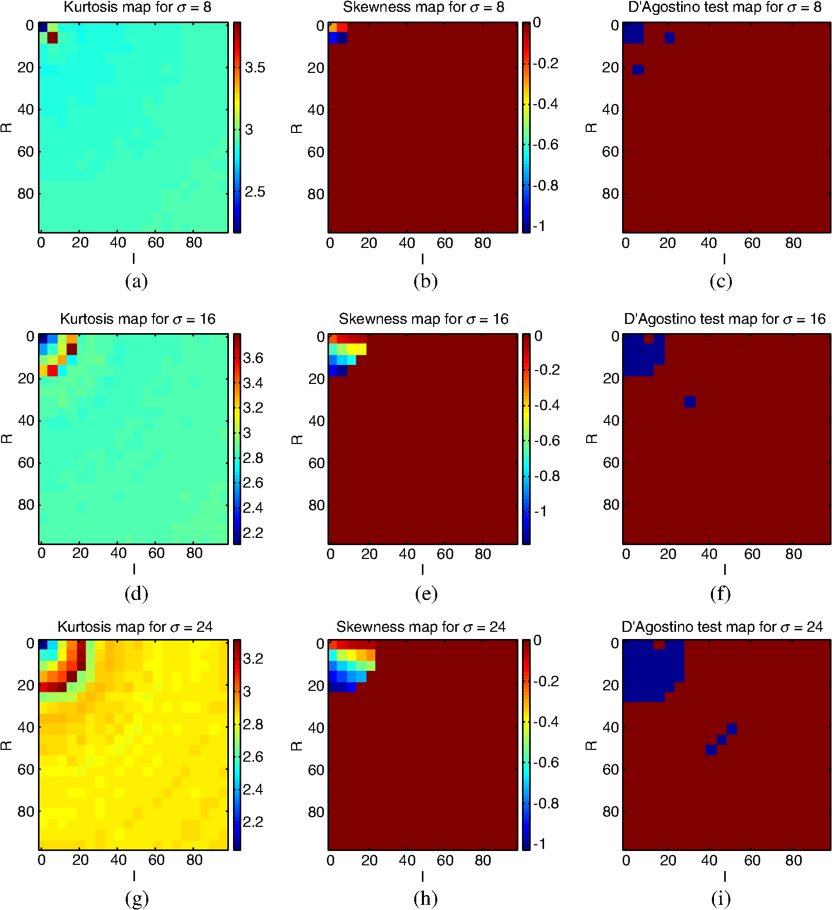

Fig. 7

(a), (c), and (e) Current density measured in $\mathrm{A}/{\mathrm{m}}^2$ when no current is injected (pseudocurrent effect), 20 mA is injected (set 1), and 45 mA injected (set 2), respectively. (b), (d), and (f) Histograms of these currents inside the phantom in a slice respectively and the fitted Gaussians (in red).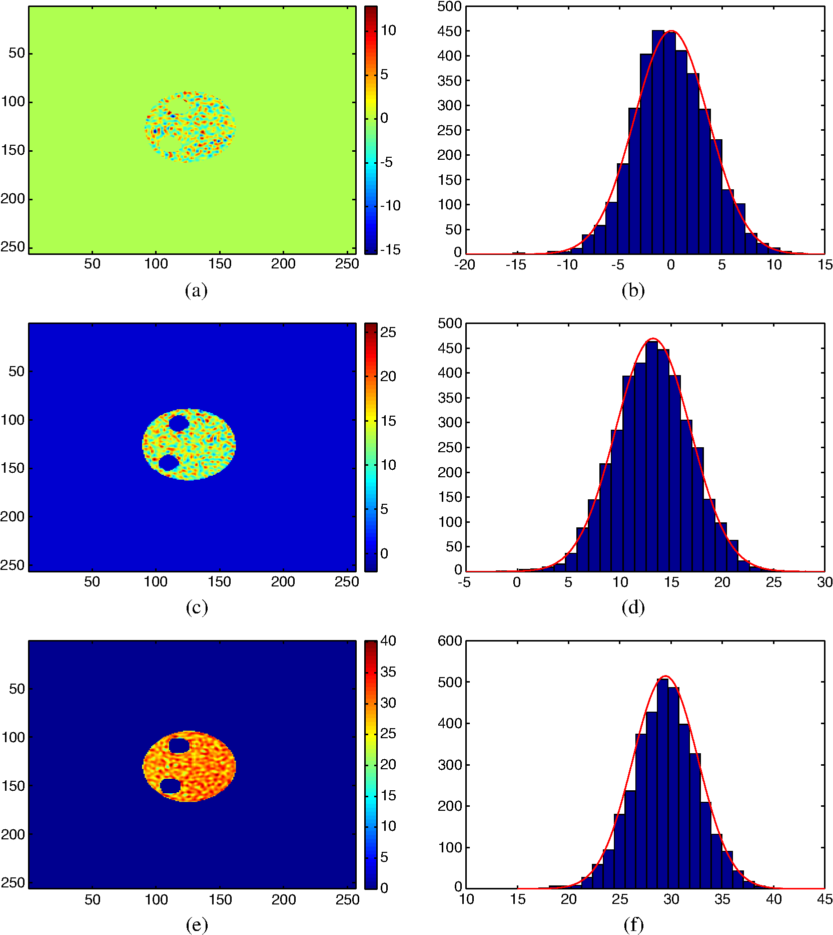

Fig. 8

(a) Probability distribution of $\theta$ [Eq. (12)], shown for pixels for various $I$s (15, 20, 25, and 30) while magnitude is constant and $\sigma$ is 8. (b) The same probability distributions from part (a) zoomed between 0 and 2 for better view.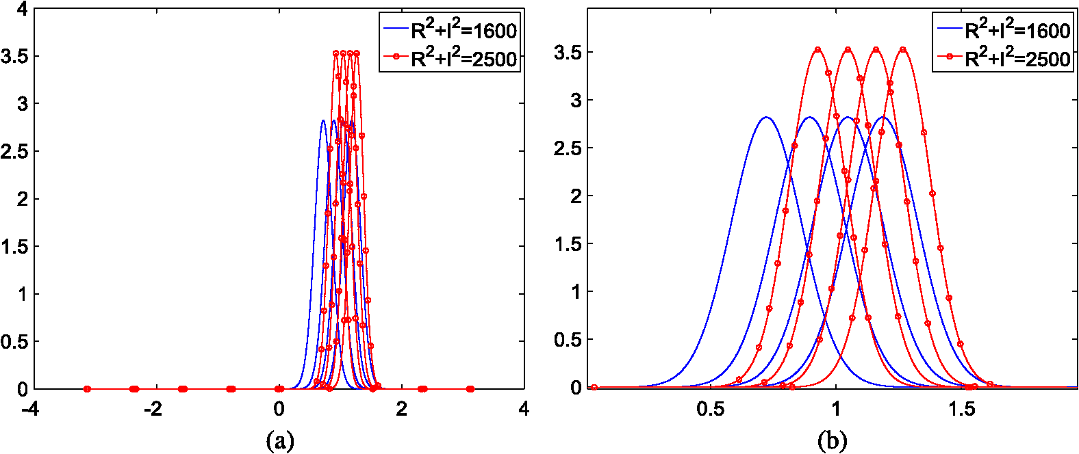

Therefore, we can conclude that the standard deviation of the noise in CDIs only depends on magnitude and for a material with an approximately constant magnitude, the noise distribution in the current density has the same Gaussian distribution for all the points. The only difference between such a subject and our phantom is that the current density values are not constant due to the lack of symmetry which translates into Gaussian distributions for current densities with the same standard deviation and the mean determined by the non-noisy current density value at that point. The standard deviation of this noise can be experimentally found for each magnitude level.

3.

Results and Discussion

In evaluating the denoising performance of the techniques, SSE on the normalized current values was used. The measured currents were normalized for ease of comparison between the two datasets. To remove the unreliable points from the edges, the final measured $J$s were eroded on the boundaries. This erosion causes the loss of some area of the phantom in the imaging slices. In this analysis, we lost 19% of the area due to erosion, therefore, the total measured (expected) current was around 16.2 mA for Dataset 1 and 36.5 mA for Dataset 2. Figures 9 and 10 show the box plots of the SSE on the normalized current results for all scenarios in Dataset 1 and Dataset 2, respectively. The data in each box plot are from multiple CDI acquisitions (multiple slices). The measured current densities are normalized by the injected currents’ amplitudes in milliamperes and SSE is calculated between the normalized measured current densities and the normalized expected current density. The normalized expected current density is calculated by dividing 1 mA (normalized current) over the area of the phantom slice because of the uniformity of the current density in the phantom. From the SSE results, we can see that overall the BM3D method performs better in denoising CDI images than the compared existing techniques. It performs well both in applying denoising on the real and imaginary images before calculating the phase as well as on the final calculated current density map ($J$). The performance is better when the BM3D method was applied to the final measured $J$ than when it was only applied to $R$ and $I$ for both datasets. It can be noted that the normalized SSEs have higher values for lower current because of the normalization by the current amplitude; for higher currents the values will be lower. We also computed the $P$-values to demonstrate the pairwise statistical differences between SSE distributions between the techniques. The statistical significance along with a lower SSE demonstrates the pairwise comparative performance of the techniques. The $P$-values calculated between different scenarios are shown in Table 2. The $P$-values were calculated using an ANOVA 1 test²² while the null hypothesis is that the data of the compared scenarios were obtained from same dataset with the same mean. It can be seen that for both datasets the $P$-values show a significant statistical difference between PM and BM3D and also between the Wiener and BM3D scenarios. The $P$-values show more distinction for lower current values where we have a lower signal-to-noise ratio (SNR) (Dataset 1). This is expected since at lower SNRs, the real gain of denoising is emphasized and this separates the SSE distributions of the techniques.

Fig. 9

Box plot of normalized SSEs for different scenarios applied to Dataset 1.

Fig. 10

Box plot of normalized SSEs for different scenarios applied to Dataset 2.

Table 2

P-values of SSEs for various scenarios.

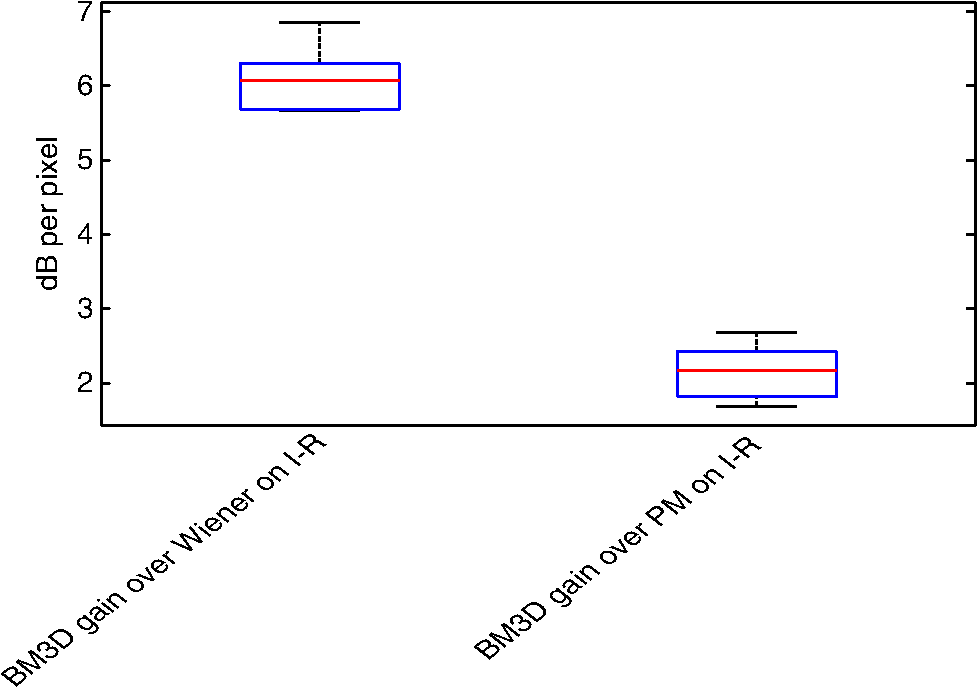
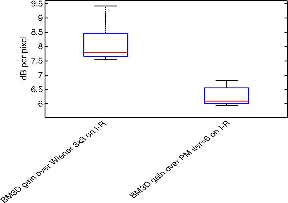
To further quantify the gains obtained by applying the BM3D method on $J$ images, we considered the BM3D result as the reference and calculated the average SSE per pixel between BM3D and the other two methods (Wiener and PM). The results are shown in Figs. 11 and 12 for both datasets. The data in each box plot are from multiple CDI acquisitions (multiple slices). The comparative gain (dB per pixel) in denoising is evident from the results. We also note that the noise suppression is higher for PM in lower SNRs (Dataset 1), while it is higher for Wiener in the higher SNRs (Dataset 2). The performance of BM3D could be attributed to the fact that it uses a sparse representation of images by exploiting the fact that there is structural redundancy and similarity in the images and that it also uses a 3-D denoising method. It reconstructs the denoised image by emphasizing the groups of patches with higher similarity. Considering that our data were acquired using a homogeneous cylindrical phantom, the structural redundancy and similarity might have aided the BM3D to some extent; further analysis in future studies using real world scenarios should be done. However, because BM3D is shown to outperform other denoising methods on standard images,¹⁵ the results can be extended to the application of CDI to tissues. Regardless of the image structure, a better denoising performance is expected from BM3D compared with the two other methods (PM and Wiener). BM3D compared with PM has a wider definition of image patterns. It deals with multiple groups of similar patches instead of only the edge or nonedge patterns dealt with in PM and on top of that it employs Wiener filtering. Comparing BM3D with Wiener filtering, we can see that although BM3D also relies on Wiener filtering, it also exploits the image pattern similarities which Wiener filtering lacks. All these denoising methods compromise the spatial resolution for the sake of combating noise. Nevertheless, the approximation of noise distribution in $J$ as Gaussian has provided with the motivation in exploring appropriate denoising methods that would optimally remove the noise influence from the current measurements.

Fig. 11

Box plot of BM3D noise suppression for Dataset 1.

Fig. 12

Box-plot of BM3D noise suppression for Dataset 2.

4.

Conclusion

The accuracy of current measurements using the CDI technique is affected by the inherent MRI noise. This noise, which is present in the initial real and imaginary images recorded by the MR scanner, is reflected in the final measured current density map. In this work, we have shown that the current density noise distribution at each pixel can be approximated by a Gaussian that depends on the noiseless values of real and imaginary images at the pixel and the variance of the background noise. Three denoising methods were evaluated at two different stages of the CDI current density measurement algorithm. Based on the obtained results using two CDI datasets of phantom images, the BM3D method which was originally designed for Gaussian noise, performs better than the other two techniques compared in this work. Furthermore, the BM3D method also performs better when applied directly on the final calculated $J$ which simplifies the denoising operation in comparison to applying it on $R$ and $I$ images.