
|
|
1.IntroductionIn 1980, digital subtraction angiography (DSA)1,2 was introduced, providing time-resolved images of a contrast injection of a vascular network. Later, in 1997, three-dimensional (3-D) DSA (Refs. 3 and 4) made possible the 3-D reconstruction of a vascular network obtained from a 3-D rotational acquisition [multiframe two-dimension (2-D) at trajectory angles]. Currently, in clinical practice, temporal dynamics of the vascular network under study must be obtained from 2-D acquisitions either from the rotational acquisition or from fluoroscopy views and the 3-D representation from the temporally static 3-D DSA. Reasons for the use of C-Arm CT systems include high spatial and temporal resolution, the ability to cover a large field of view, the ability to move the C-Arm to various view angles, and real-time fluoroscopy.5 Furthering these advances came the introduction of 4-D DSA (Refs. 6 and 7) combining the temporal information of the 2-D projections and the 3-D geometry of the 3-D DSA into a true 4-D display. The need for multiple sweeps,8 up to six bidirectional sweeps were reported, of the C-Arm CT system gantry is avoided in 4-D DSA. However, it should be noted the current requirement of a sparse 4-D DSA constraining volume makes accurate parenchymal blood flow, as reported in Ref. 8, difficult. At a minimum, 4-D DSA requires one bidirectional sweep and a single injection of contrast medium. 4-D DSA provides a time series of 3-D volumes and time attenuation curves (TAC) for reconstructed voxels at the acquisition frame rate. Time-of-arrival (TOA) metrics for time to peak and time to a percent of max can be calculated using the TAC data. Using time to percent max as a metric, a true 4-D view of the 2-D parametric color coded views described in Ref. 9 can now be obtained. Both a 4-D static TOA (3-D) and 4-D dynamic TOA (4-D bolus arrival) can be achieved.7 The 4-D DSA reconstruction allows the viewing of the ROI volume at any time from any angle and from any angle at any time. 4-D DSA avoids the unobtainable view problem inherit in 2-D DSA fluoroscopy due to gantry collisions with patient or couch. Current research10 indicates 4-D DSA can provide superior visualization of the temporal dynamics of the draining and filling vascular networks extending from the nidus of arterovenous malformations (AVMs); however, further experience is needed with the technique. There is also indication that 4-D DSA can be used to obtain insight into the angioarchitectural features of an AVM. The ability to use the temporal views of 4-D DSA can be seen in Fig. 1. Fig. 1On the left is a 3-D DSA of a canine with all vessels opacified. On the right is a 4-D DSA early time frame before opacification of the venous return vessels. Demonstrated is the ability of 4-D time frames to provide an unobstructed view of arterial vessels. The 3-D DSA contains both arteries and veins, therefore obscuring visualization of the internal carotid arteries (ICAs). The white arrows highlight the course of the right ICA in the 4-D DSA view. The ellipse highlights the distal segments of the ICAs for reference. Both these reconstructions can be viewed from any angle; however, only 4-D DSA can be viewed from any time. 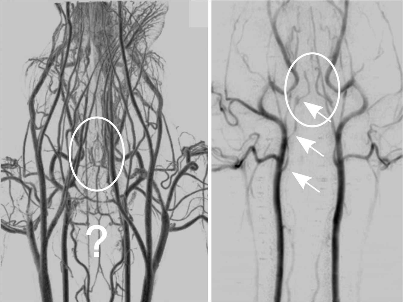 The purpose of this research was to investigate the volumetric spatial resolution of the time series of 4-D DSA reconstructions when varying reconstruction parameters specific to the 4-D DSA algorithm. The parameters varied were the 2-D projection blurring kernel size and the threshold applied to the C-Arm CT Feldkamp, Davis, and Kress (FDK) reconstruction (3-D DSA). The kernel affects the spatial resolution and signal-to-noise ratio (SNR) of the projection, while the threshold affects the spatial resolution and SNR of the 3-D volume used as a constraining image. 4-D temporal volume spatial resolutions were then compared to the 3-D DSA. Results were determined for both physical phantom and in silico phantom (ISPH) and compared to the 3-D DSA. This research was performed under both an institutionally approved animal care and use committee protocol for animals and an IRB protocol for human data. 2.Methods2.1.Four-Dimensional Digital Subtraction Angiography4-D DSA is made possible by combining the 3-D DSA volume and the 2-D rotational projections containing temporal information using the 4-D DSA algorithm further discussed in Fig. 2 and described by Eqs. (1) and (2). The projection sampling of a C-Arm CT system is shown in Eq. (1), where is the sampling period. The constraining image, , is first generated by applying a threshold to the 3-D DSA volume. A projection containing temporal information, , is convolved using the operator “*” with a 2-D square blurring kernel, , of uniform intensity. The forward projection of the constraining image is also blurred by the kernel . The convolution of projections acts to increase SNR (Ref. 7) of the projection image. These projection data are then divided element by element and backprojected, , into 3-D space at the view angle to create a weighting volume . The operator backprojects a projection value at detector coordinates and to a 3-D coordinate , , and in 3-D space given the view angle . The backprojection operation does not perform any filtering or weighting of the projection data. This work implemented the p-matrix voxel driven backprojection algorithm as described in Scherl et al.,11 Wiesent et al.,12 and Galigekere et al.13 The Hadamard product “” of the weighting volume, , and the constraining image, , generates raw 4-D time frame, , data, which can be further processed. The postprocessing includes corrections for vessel overlap in a projection, which causes a reconstruction artifact, higher than actual values during overlap periods, in the TACs of 4-D DSA.Fig. 24-D reconstruction process illustrating the projection space left of the dashed line and 3-D space on the right. The projections are first acquired in step 1. The volume is then reconstructed from projections as shown in step 2. Constraining image generation by which the 3-D DSA is threholded is shown in step 3. The 2-D blurring kernel is applied to the temporal projections and reprojections (not shown) of the constraining volume in step 4. The blurred temporal projections and reprojections are then divided (not shown). The normalized projections are then backprojected individually to create a weighting volume for each time frame, step 5, and the result is multiplied with the constraining image shown in step 6. Highlighted are steps 3 and 4 as the effect these steps have on the limiting spatial resolution is the focus of this research.  The 2-D projections record the contrast enhanced dynamics of the vascular network under study following the single injection of contrast near the start of the acquisition. The 2-D projections are used to generate the 3-D DSA volume through conventional techniques.12,14 The 3-D DSA volume is then sparsified using a simple thresholding approach to generate a 3-D volume for use as a volumetric constraining image, . Constraining volume generation using 3-D DSA has the effect of removing background noise, thus allowing the viewing of the vascular network. The process is similar to that of window and leveling techniques currently used to view current 3-D reconstruction volumes. The angle represents the scan acquisition trajectory view angle at the acquisition time frame . There is a direct relationship between the projection angle and the time index ; therefore, the terms will be used interchangeably. For forward projections, of the constraining image are taken at the same angle as the temporal projection . The constraining image, , is a static image with no temporal variation, where has no meaning other than to simplify the equations and shall be equivalent to . The equations, descriptive geometry, and reconstruction algorithm for 3-D DSA are discussed in numerous sources, notably Refs. 12 and 14. The 3-D DSA reconstruction process involves cosine weighting, Parker-weighting,15 and convolution of the projections with a one-dimensional (1-D) filtering kernel followed by a backprojection into 3-D space. Convolution occurs only along the dimension perpendicular to the axis of rotation and is not a 2-D convolution. The 3-D DSA and 4-D DSA reconstructions used the same 1-D Hamming filter as the 4-D DSA constraining image is derived from the 3-D DSA. The convolved temporal and constraining projections have a consistent attenuation where vessels occur. However, due to vessel overlap in a given projection, attenuation is increased in overlap areas, which creates artifacts in the per voxel TAC of 4-D DSA when reconstructed. To mitigate this effect, the convolved temporal projections are then normalized by dividing the constraining projections element by element to aid in minimizing artifacts due to vessel overlap to create the normalized 2-D temporal time frame projection as shown in Eq. (3). Normalization does not completely eliminate overlap as the constraining image is a time average integral through the vessels. What is ultimately desired out of the division process is a normalized projection in the set of real numbers, and . An ideal normalized projection allows the activation or deactivation of the vessel network in the constraining image when backprojected to create the weighting image. In practice, this is challenging to obtain as the constraining volume is a time average of the reconstructed temporal projections. Thus, the reprojection of the constraining image is a projection of a time averaged volume. Normalization allows the weighting of the image by a factor between zero (off) and one (on). A method found to work is described in Eq. (4). The denominator is increased by a factor that is five percent of the max value of the projection data in the denominator. While normalization of the projections can aid in decreasing the vessel overlap artifact, algorithms have been created to further reduce the artifact. The single projection (SP) algorithm described in Eq. (2) is the basic algorithm of 4-D DSA. It became clear early on in the investigation of 4-D DSA that this algorithm would require further refinement to account for vessel overlap in the projections. 4-D DSA separation angle (SA) and minimum within a search angle (MSA) algorithms have been developed to further process the 4-D data generated by Eq. (2) temporally on a voxel-by-voxel basis.The separation angle algorithm is described in Eq. (5) and takes two projections separated by an angle. The square root is used as an approximation to retain the actual values as two projections and thus two weighting volumes are used. A typical value for was one that would yield an angular separation in the acquisition trajectory of 30 deg. The SA is selected to provide a physical projection angle separation while still maintaining acceptable temporal resolution. Ideally, the angle selected would be 90 deg, providing ideal spatial separation; however, selecting this value is at the cost of temporal resolution. The minimum search angle algorithm as described by Eq. (6) aims to decrease vessel overlap artifacts by searching for the minimum value of the temporal data for a given voxel over a search angle to mitigate the contrast curve intensity spikes that can occur when vessels overlap in a projection. The value is the minimum temporal index over a time range , where the argument minimum of is at a minimum on a per voxel TAC basis. The case as approaches the last temporal index , the temporal delta is allowed to approach zero, , as the number of remaining time frames decrease. For a given voxel TAC, the time index selected for the time frame is the time frame with the lowest TAC value. This time index thus selects the lowest TAC value over the search range. Thus, represents a 3-D array of time indices for each voxel TAC where the value in each voxel TAC is a minimal value over the temporal search range.While in an ideal mathematical sense MSA is equivalent to SP and SA algorithms when a perfect static object is used, when used in real-world data, this is not the case due to imperfections in scan geometry and data acquisition. However, limiting spatial resolution results for the other algorithms were found to be identical to the results of MSA. The effects of the algorithms were not the focus of this research. Recently, various interpolation algorithms have been developed and investigated to interpolate over areas of vessel overlap in the TAC data. The impact of these interpolation algorithms on resolution were not investigated in this work. 2.2.Frequency ResponseA simplified form of the equation for 4-D DSA is shown in Eq. (7). The division by the reprojection of the constraining volume has been omitted for the current purposes of discussion; the theta notation and time variable have been dropped for the sake of simplicity. The notation shown shall use lowercase to represent equations in image space with uppercase variables representing the Fourier transformed variables in frequency space. The temporal projection data, , is first convolved with the blurring kernel, . This operation is a convolution in image space, but is a multiplication in frequency space as described by Eqs. (8), (9), and (10). This is essentially a low-pass filter operation in which frequency content in the projection is limited to the bandwidth of the filter kernel . Basic properties of MTF and frequency analysis will be used to discuss the effects of 4-D DSA on the limiting spatial resolution. The equation 16 using the Fourier transform, , for finding the MTF given the point spread function (PSF) data is shown in Eq. (11). The solution for the MTF of the system is shown in Eqs. (12) and (13). For the purpose of discussion, the limiting spatial resolution of two data sets in object space, and , having been transformed into frequency space, and , shall be defined here as and , respectively. The maximum limiting spatial frequency resulting from product of the two frequency responses is defined in Eq. (14). The limiting spatial resolution in MTF analysis is either the point where the MTF reaches the first zero when using a pure mathematical approach or in analysis of real-world data, the first point on the MTF curve that reaches 10% of the value at zero spatial frequency starting from zero spatial frequency. The maximum limiting spatial frequency, , of a convolution operation in image space is the minimum of the spatial frequency of the data being convolved, sets and , as the multiplication in frequency space is dependent on the first zero crossing of either of the two data sets as described by Eq. (14). The limiting spatial frequency for the resulting 4-D DSA temporal projection, , to be backprojected is therefore described by Eq. (15). The next step is to backproject the temporal projection, , to the object plane. The scaling of the image detected by the detector at the image plane is scaled into the object plane and is accomplished through the backprojection operation. The magnification, , represents the geometric scaling factor. The backprojection operation is not a simple 1-D operator, but acts to project the data along direct rays between the image plane and the source. However, for the purposes of discussion and to aid in clarity of understanding the backprojection operation effects on 4-D DSA, the backprojection operation shall be represented as a scaling of image data to the object plane. This analysis is akin to taking a 1-D centered radial sample of the transverse plane such that at the angle that is acquired, the central slice object data axis is exactly parallel with the detector as shown in Fig. 3.The effect of this is shown as scaling the projection of an object of width from the image plane to the object plane , as shown in Fig. 3, resulting in an object width of . This results in a frequency scaling in frequency space and is described by Eq. (16) and application to 4-D DSA in Eq. (17). The last operation to be performed is that of multiplying the constraining image with the backprojection of the temporal projection. A multiplication in image space is a convolution in frequency space. The wire object in the constraining image and the weighting volume image were modeled with a pair of Jinc functions17 to aid in determining the effects of the multiplication in image space. Various sizes were used in the model and resulted in the maximum spatial frequency tracking with object that had the highest spatial frequency or the smaller of the two objects in image space. Therefore, it was determined that maximum spatial frequency of the multiplication of the constraining image with the weighting volume is the maximum of the two spatial frequencies of the two objects when convolved in frequency space as described by Eq. (18) and with application to 4-D DSA shown in Eq. (19). The resulting limiting resolution of 4-D DSA, , is the maximum of the limiting resolution of the constraining image, , and the minimum of the limiting resolution of the blurring kernel and the temporal projection data, , scaled to the image plane by the scale factor, , as shown in Eq. (20). The 4-D DSA process includes a number of nonlinear operations such as thresholding and division of the temporal projections by reprojections of the constraining volume. Although 4-D DSA is a nonlinear system, it is treated as linear at an operating point. The standard approach18 of scanning a fine highly attenuating wire centered in and perpendicular to the transverse plane was performed. The effects of the 4-D DSA reconstruction on volumetric spatial resolution were investigated using both an ISPH and the scan of a physical 76 micron (um) diameter tungsten wire centered in a cylindrical supporting structure. ISPH was modeled after the PPH as cylinder centered in the transverse plane with the axis parallel to the axis of rotation extending throughout the entire volume of interest. The physical phantom is shown in Fig. 4. The constraining image inherits the reconstruction parameters from the 3-D DSA as it is a 3-D DSA where a threshold has been applied. The spatial resolution of a 4-D temporal volume can be obtained by the same means as for the 3-D DSA. The 3-D DSA is compared with the 4-D temporal frames (temporally enhanced 3-D volumes) of 4-D DSA reconstructions. This was done on a volumetric basis using a single transverse slice of a physical or digital phantom of a small wire. Resulting PSF data were radially averaged and Fourier analysis performed to generate averaged MTF data for each 3-D DSA volume and 4-D DSA temporal slice. The limiting spatial resolution was automatically determined by finding the spatial resolution when 10% of the magnitude at zero spatial frequency was reached. Numerical simulations and reconstruction of the real-world phantom were performed using a combination of MATLAB® (The Mathworks Inc., Natick, Massachusetts) and CUDA (NVIDIA Corp. Santa Clara, California) based software. The spatial resolution at the center of the central slice of the C-Arm CT biplane system (Artis zee, Siemens Healthcare, Forchheim, Germany) used is determined by Eq. (21) and is based on the Nyquist sampling criteria using the detector spacing (), imaging geometry source to image distance (SID), and source to object distance (SOD) to determine the minimal detectable distance achievable in the transverse plane. This equation does not account for blurring effects due to focal spot, geometric instabilities of the C-Arm, or projection filtering. The minimal resolvable distance calculation is shown in Eq. (22). The scan geometry was determined using a standard 4-D DSA acquisition procedure without zoom of the detector/C-Arm with SID set to the maximum of 1200 mm and SOD held constant at 750 mm resulting in the magnification factor , and collimation set to maximum field of view with binning yielding a detector resolution of detector elements with isotropic detector element size of 0.3080 mm ( native nonbinned resolution with 0.154 mm isotropic detector elements). The minimal resolvable distance is calculated with Eq. (22), which was used to ensure the reconstruction grid was smaller than this dimension. The selection of the maximum allowable wire size was found to be 86 micron using the approach of Nickoloff.19 The reconstruction grid (slice) was 512 by 512 voxels with a 0.0376 mm isotropic voxel size. The voxel size was made considerably smaller than the minimum resolvable object size, , to ensure proper reconstruction and 4-D DSA reconstruction artifacts could be properly investigated. Off axis and off central slice resolution was not investigated in this research and is a topic for future investigation and research. The physical wire phantom was built using a Scientific Instruments (New Jersey) 0.076 mm tungsten wire part number W91 surrounded in an air-filled thin-walled plastic cylinder, 47 mm O.D., as a supporting structure as shown in Fig. 3. The phantom was then scanned on C-Arm CT biplane system. The scan procedure was 8.2 s in duration providing 248 projections, at a frame rate of 30 fps, at 60.4 kVp and 168 mAs.Fig. 4Image of the physical phantom. The location of the tungsten wire has been highlighted by dark gray box overlaid on the image and is located in the center of the box.  The phantom was placed in the field of view for the mask run and removed from the field of view for the fill run. This was done to allow the same processing pipeline to be used for current 4-D DSA processing while also setting the automatic exposure control to the object during the mask run. The mask and fill projections were then interchanged to allow correct subtraction and sign of the value in the projections. Normalized projections using Eq. (4) were used in this analysis. The steps to generate MTFs are as follows. Select a backprojection filtering kernel and perform a reconstruction at the correct zoom factor to satisfy the Nyquist criteria and reconstruction grid requirements. Acquire a central transverse slice of the temporal frame of the reconstructed object and repeat the process for each 4-D volume. Sum all transverse slice time frames extracted from each 4-D time frame volume to make a composite PSF. Find the center of the composite PSF. Preprocess the transverse slices of the temporal time frame if necessary. Radially average the temporal slice in the spatial domain using the center coordinates found using the composite time frame. Generate the measured modulation transfer function (MTF) from the radially averaged PSF by taking the fast Fourier transform (FFT). Then take the absolute value of the result of the FFT. The system MTF is then determined by dividing the measured MTF by an estimate of the MTF of the object (Jinc). The maximum spatial resolution is determined from the resulting MTF plot by finding the first zero or value on the frequency axis where a ten percent of the zero frequency value is reached. Generation of a composite frame stated above was performed to aid in finding an accurate center of the PSF. Composite frame generation was performed to avoid projection angle dependent modulation in some reconstructed frames. The modulation was induced by the backprojection of blurred temporal projection data where blurring as a result of the blurring kernel, of size zero or two, is less than that induced blurring due to geometric instability. Preprocessing of the transverse slice as stated above can include cropping the image from 512 to 64 voxels on center to avoid any ripples in the frequency response curve near zero spatial frequency due to the standard deviation increasing with increasing as described in Ref. 17. 3.ResultsThe limiting spatial resolution of the 3-D DSA was found to be higher for ISPH than for PPH and is a result of simulated processing stage not accounting for geometric instability and focal spot blurring. While these results are not similar, the discussion of the differences is an important topic. The results are summarized in Table 1. Frequency response plots for the 3-D C-Arm CT, constraining image, PPH, and ISPH are shown in Figs. 5, 6(a), and 6(b). Table 1ISPH and PPH limiting spatial resolution summary table.
Fig. 6Frequency response results for the (a) ISPH and (b) PPH. Near-exact results have been grouped for clarity. 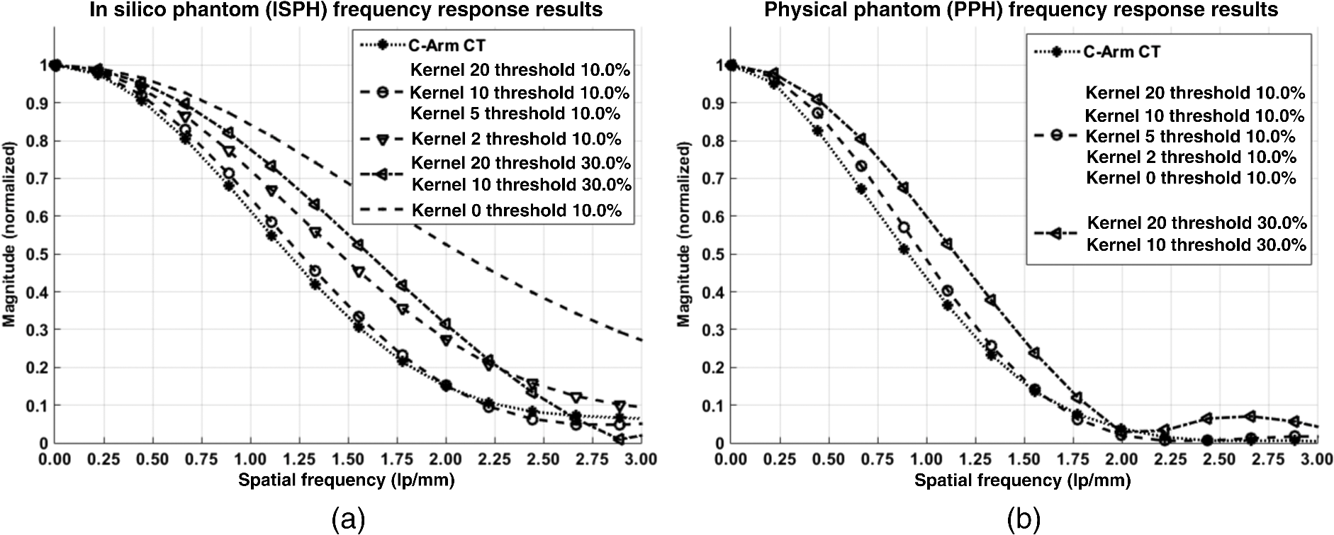 The spatial resolution of the 4-D DSA tracks with that of the constraining image as can be seen from the table when appropriate kernel sizes, 5, 10, and 20, are used. Provided the threshold of the constraining image is not severe and limiting resolution of the constraining image is maintained close to the 3-D DSA, the limiting resolution of 4-D DSA temporal volumes are very near to the resolution of the 3-D DSA reconstruction volume. While Eq. (20) may appear to inflate the resolution of 4-D DSA, it does so only marginally. Blurring kernels of the size typically used widen the object data in image space and thus decrease the limiting spatial frequency of the object in frequency space. The wider the image is in image space, the smaller the value is for the zero crossing in frequency space for the frequency response of the image and, thus, the smaller the contribution is to the resulting limiting spatial resolution. When typical parameters for the projection blurring are used, the effects of the weighting volume term () in Eq. (20) has little impact on the limiting spatial resolution. When the 4-D DSA algorithm is applied with square kernels of 5, 10, and 20 pixels, the resolution is lowered for ISPH and PPH only as a result of the constraining image. The kernel size can only act to increase the resolution beyond the constraining image by allowing high spatial frequency data in the projection to modulate the constrain image. This represents a reduction of for ISPH and for PPH. These typical values for the kernel size have a minor effect on the spatial resolution. It is not until the kernel is changed to 2 or no kernel is applied that projection is allowed to retain the high spatial frequency content. The effect is a modulation of the 4-D DSA volumes during the backprojection operation. The result is a narrowing of the 2-D PSF of the constraining 3-D volume perpendicular to the ray along which the data are backprojected. Figures 7 and 8 clearly show when modulation does and does not occur along the projection. Figures 7(b) and 9(b) demonstrate the modulation at the projection angle. This acts to cause an inflation of the results for the 4-D limiting spatial resolution as described by Eq. (20). The effect is apparent only in ISPH due to the ideal reconstruction process and the retention of high spatial frequency content in the projections. Modifying the volume threshold has the expected effect of artificially inflating the limiting resolution as can be seen when comparing datasets for which the kernel size was 10 or 20 and the threshold changed from 10 to 30% for either phantom. Fig. 7ISPH profiles of the PSF with (a) kernel size 5 and 10% threshold and (b) kernel size 0 and 10% threshold.  4.Conclusion4-D DSA is capable of producing a time series of 3-D angiographic volumes that have occurred at any time in the scan and from any view angle while retaining the resolution of the C-Arm CT FDK reconstruction (3-D DSA) volume. 4-D DSA is capable of providing a resolution of at a temporal resolution of 30 frames per second using a standard protocol. AcknowledgmentsWe would like to thank Dr. Charlie Strother for his role in the conception of the 4-D DSA technique and for his critical role in guiding of this research. Research reported in this publication was supported by the National Heart, Lung, and Blood Institute (NHLBI) of the National Institutes of Health under award number R01HL116567. The content is solely the responsibility of the authors and does not necessarily represent the official views of the National Institutes of Health. ReferencesC. A. Mistretta and A. B. Crummy,
“Diagnosis of cardiovascular disease by digital subtraction angiography,”
Science, 214 761
–765
(1981). http://dx.doi.org/10.1126/science.7292009 SCIEAS 0036-8075 Google Scholar
R. A. Kruger et al.,
“A digital video image processor for real-time x-ray subtraction imaging,”
Opt. Eng., 17
(6), 176652
(1978). http://dx.doi.org/10.1117/12.7972299 Google Scholar
R. Fahrig, M. Moreau and D. W. Holdsworth,
“Three-dimensional computed tomographic reconstruction using a C-Arm mounted XRII: correction of image intensifier distortion,”
Med. Phys., 24
(7), 1097
–1106
(1997). http://dx.doi.org/10.1118/1.598013 MPHYA6 0094-2405 Google Scholar
R. Fahrig et al.,
“Use of a C-Arm system to generate true three-dimensional computed rotational angiograms: preliminary in vitro and in vivo results,”
Am. J. Neuroradiol., 18
(8), 1507
–1514
(1997). Google Scholar
R. Gupta et al.,
“Ultra-high resolution flat-panel volume CT: fundamental principles, design architecture, and system characterization,”
Eur. Radiol., 16 1191
–1205
(2006). http://dx.doi.org/10.1007/s00330-006-0156-y EURAE3 1432-1084 Google Scholar
C. A. Mistretta et al.,
“4D-DSA and 4D fluoroscopy: preliminary implementation,”
Proc. SPIE, 7622 762227
(2010). http://dx.doi.org/10.1117/12.844561 Google Scholar
B. Davis et al.,
“4D digital subtraction angiography: implementation and demonstration of feasibility,”
Am. J. Neuroradiol., 34
(10), 1914
–1921
(2013). http://dx.doi.org/10.3174/ajnr.A3529 Google Scholar
A. Ganguly et al.,
“Cerebral CT perfusion using an interventional C-Arm imaging system: cerebral blood flow measurements,”
Am. J. Neuroradiol., 32 1525
–1531
(2011). http://dx.doi.org/10.3174/ajnr.A2518 Google Scholar
C. M. Strother et al.,
“Parametric color coding of digital subtraction angiography,”
Am. J. Neuroradiol., 31 919
–924
(2010). http://dx.doi.org/10.3174/ajnr.A2020 Google Scholar
C. Sandoval-Garcia et al.,
“4D DSA a new technique for arteriovenous malformation evaluation: a feasibility study,”
J. Neurointerv. Surg., 011534
(2015). http://dx.doi.org/10.1136/neurintsurg-2014-011534 Google Scholar
H. Scherl et al.,
“Evaluation of state-of-the-art hardware architectures for fast cone-beam CT reconstruction,”
Parallel Comput., 38 111
–124
(2012). http://dx.doi.org/10.1016/j.parco.2011.10.004 PACOEJ 0167-8191 Google Scholar
K. Wiesent et al.,
“Enhanced 3-D-reconstruction algorithm for C-Arm systems suitable for interventional procedures,”
IEEE Trans. Med. Imaging, 19 391
–403
(2000). http://dx.doi.org/10.1109/42.870250 ITMID4 0278-0062 Google Scholar
R. R. Galigekere, K. Wiesent and D. W. Holdsworth,
“Cone-beam reprojection using projection-matrices,”
IEEE Trans. Med. Imaging, 22 1202
–1214
(2003). http://dx.doi.org/10.1109/TMI.2003.817787 ITMID4 0278-0062 Google Scholar
L. A. Feldkamp, L. C. Davis and J. W. Kress,
“Practical cone-beam algorithm,”
J. Opt. Soc. Am., 1
(6), 612
–619
(1984). http://dx.doi.org/10.1364/JOSAA.1.000612 Google Scholar
D. L. Parker,
“Optimal short scan convolution reconstruction for fan beam CT,”
Med. Phys., 9 254
–257
(1982). http://dx.doi.org/10.1118/1.595078 MPHYA6 0094-2405 Google Scholar
Jerrold T. Bushberg, The Essential Physics of Medical Imaging, 2nd ed.Lippincott Williams & Wilkins, Philadelphia
(2002). Google Scholar
C. J. Bischof and J. C. Ehrhardt,
“Modulation transfer function of the EMI CT head scanner,”
Med. Phys., 4
(2), 163
–167
(1977). http://dx.doi.org/10.1118/1.594305 MPHYA6 0094-2405 Google Scholar
W. Kalender, Computed Tomography: Fundamentals, System Technology, Image Quality, Applications, MCD Verlag, Germany
(2000). Google Scholar
E. L. Nickoloff,
“Measurement of the PSF for a CT scanner: appropriate wire diameter and pixel size,”
Phys. Med. Biol., 33 149
(1988). http://dx.doi.org/10.1088/0031-9155/33/1/014 PHMBA7 0031-9155 Google Scholar
BiographyBrian J. Davis is a PhD candidate studying biomedical engineering at University of Wisconsin–Madison. He received his bachelors in electrical engineering with computer option at Bradley University in Peoria, Illinois, in 1999 and his MS degree in biomedical engineering at University of Wisconsin–Madison in 2011. His interests include medical imaging, aerospace research and development, image processing, embedded systems, and human machine interfaces. He is a member of SPIE. Erick Oberstar is a PhD dissertator in the Biomedical Engineering Department as well as a faculty associate in the Mechanical Engineering Department running the Mechatronics Laboratory, at University of Wisconsin–Madison. He received his bachelors in electrical engineering at University of Wisconsin–Platteville and his MS in electrical engineering (signal processing & controls) from University of Wisconsin–Madison. He has extensive cross-disciplinary design experience including medical imaging, mechatronics, embedded systems, signal processing, and controls. Kevin Royalty is currently the director of Angiography Research Collaborations for the Eastern USA with Siemens Medical Solutions USA Inc. He has degrees in electrical engineering, biomedical engineering, and business administration, and has worked in the defense industry, telecommunications industry, venture capital, and most recently the medical device industry. He is a member of SPIE. |
|||||||||||||||||||||||||||||||||||||||||||||||||||||||||||||||||||||||||||||||||||||||||||||||||||||||||||||||||||||||||||||||||||


