Variability and accuracy of different software packages for dynamic susceptibility contrast magnetic resonance imaging for distinguishing glioblastoma progression from pseudoprogression

Zachary S. Kelm; Panagiotis D. Korfiatis; Ravi K. Lingineni; John R. Daniels; Jan C. Buckner; Daniel H. Lachance; Ian F. Parney; Rickey E. Carter; Bradley J. Erickson

doi:10.1117/1.JMI.2.2.026001

26 May 2015 Variability and accuracy of different software packages for dynamic susceptibility contrast magnetic resonance imaging for distinguishing glioblastoma progression from pseudoprogression

Zachary S. Kelm, Panagiotis D. Korfiatis, Ravi K. Lingineni, John R. Daniels, Jan C. Buckner, Daniel H. Lachance, Ian F. Parney, Rickey E. Carter, Bradley J. Erickson

Author Affiliations +

Journal of Medical Imaging, Vol. 2, Issue 2, 026001 (May 2015). https://doi.org/10.1117/1.JMI.2.2.026001

Abstract

Determining whether glioblastoma multiforme (GBM) is progressing despite treatment is challenging due to the pseudoprogression phenomenon seen on conventional MRIs, but relative cerebral blood volume (CBV) has been shown to be helpful. As CBV’s calculation from perfusion-weighted images is not standardized, we investigated whether there were differences between three FDA-cleared software packages in their CBV output values and subsequent performance regarding predicting survival/progression. Forty-five postradiation therapy GBM cases were retrospectively identified as having indeterminate MRI findings of progression versus pseudoprogression. The dynamic susceptibility contrast MR images were processed with different software and three different relative CBV metrics based on the abnormally enhancing regions were computed. The intersoftware intraclass correlation coefficients were 0.8 and below, depending on the metric used. No statistically significant difference in progression determination performance was found between the software packages, but performance was better for the cohort imaged at 3.0 T versus those imaged at 1.5 T for many relative CBV metric and classification criteria combinations. The results revealed clinically significant variation in relative CBV measures based on the software used, but minimal interoperator variation. We recommend against using specific relative CBV measurement thresholds for GBM progression determination unless the same software or processing algorithm is used.

1. Introduction

Glioblastoma multiforme (GBM) is the most common adult, primary brain cancer and carries a poor prognosis. Median survival in patients treated on clinical trials with radiation therapy and temozolomide ranges from 15 to 20 months.¹^,² After biopsy or maximal safe resection, patients typically receive $\sim 60 Gy$ of radiation over 30 fractions, concurrent with daily low-dose temozolomide. Patients then go on to receive adjuvant temozolomide for 6 to 12 months or longer, while being imaged every two to three months to assess tumor status. If it is determined that the tumor is progressing, second-line agents are introduced. However, progression can be difficult to confidently determine based on imaging, since a treatment response can transiently cause a similar imaging appearance as tumor progression,³ often referred to as pseudoprogression. It is important to distinguish the two conditions. If there is true progression, a second-line agent may extend survival. If there is pseudoprogression, there may be a survival advantage⁴ and temozolomide should not be discontinued. It is difficult to distinguish pseudoprogression versus tumor progression by clinical symptoms, especially early in the postradiation period.⁵

In a study examining the incidence of progression versus pseudoprogression in 63 GBM patients,⁵ 28 (44.4%) of the patients had lesion enlargement with the first postradiation follow-up MR exam. Each of these cases underwent salvage surgery and pathologic analysis, resulting in 12 (42.8%) being classified as pseudoprogression, with the other 16 (57.2%) exhibiting true tumor progression. In the largest study regarding conventional imaging of progression versus pseudoprogression, qualitative features were analyzed regarding their ability to distinguish between the two phenomena.⁶ With 63 progression and 30 pseudoprogression patients, the only feature found to have predictive value regarding progression was subependymal enhancement. However, this was only present in 26 of the 93 cases, producing a negative predictive value of 41.8%, and is not a good candidate for attempting to extract further value through quantitative assessment since a radiologist would not have trouble recognizing this and determining it to be new tumor growth.

Relative cerebral blood volume (rCBV) has attracted much interest as a functional measurement potentially representing tumor-related vascular changes beyond those visible in conventional MR characteristics.⁷ In addition to many studies investigating its utility in distinguishing between tumor grades, various studies have analyzed its use in distinguishing between tumor progression and pseudoprogression. The mean rCBV in progression is higher than the mean rCBV in pseudoprogression, consistent with the understanding that active tumor elicits angiogenesis and consequently higher blood volumes. Accordingly, many authors have reported optimal rCBV thresholds for separating progression from pseudoprogression cases.⁸^–¹¹

CBV images are generated through postprocessing of a perfusion-sensitive image acquisition, which tracks signal change over time due to the transit of a contrast bolus. Dynamic susceptibility contrast (DSC) MR is commonly used to produce the perfusion-weighted images in brain tumor imaging. The CBV for each voxel is calculated based on an integral of the relaxivity change (derived from the MR signal using the echo time) measured during bolus transit from a prebolus baseline level (see Fig. 1). The starting and ending time points of this integration, baseline estimate, model fitting, integration method used, and correction for contrast agent extravasation are sources of variation in CBV calculation.¹²^,¹³ As a measurement with arbitrary units, the need for normalization has been investigated, with the most common approach being to divide by the mean contralateral white matter value to produce relative or rCBV values.¹⁴ Efforts have been made to correct the DSC signal corruption caused by contrast agent extravasation due to blood brain barrier disruption, both by bolus preload dose administration and correction using mathematical models during the CBV calculation.¹³ Previous studies have shown that both preload dosing and modeling are needed for maximal rCBV accuracy.¹²^,¹⁵ If these methods are insufficient to correct for the variability, then there is no translatability of results between studies using different software packages. The potential for variability has been recognized,¹²^,¹⁶ with recent reports of variability in measurements of mean rCBV between FDA-cleared software packages using clinical DSC-MR images.¹⁷^,¹⁸

Fig. 1

Example of the change in relaxivity versus time curve for an individual tumor voxel. The change in relaxivity reflects the concentration of gadolinium-based contrast present within the voxel. The shaded region represents the basis of cerebral blood volume (CBV) calculation.

The purpose of this study was to determine whether there were significant differences in multiple rCBV metrics from the same DSC-MR images between three FDA-cleared software packages, and if so, how much disagreement there exists at various thresholds of rCBV used to predict tumor progression. Then, using clinical or outcome-based information to classify whether the analyzed tumors were progressing or not, we investigated whether one software performed better than others for distinguishing between GBM progression and pseudoprogression. Finally, we analyzed whether there are clinically significant differences between the optimal rCBV metric thresholds found for each software.

2. Materials and Methods

2.1.

Patients

Our institutional review board reviewed and approved this retrospective study and granted a waiver of informed consent. The patient image files were anonymized prior to processing.

We identified the set of potential subjects through a medical record query for patients who had been treated at this institution with radiation and had a histologic diagnosis of GBM (SNOMED Code: M-94403). From this initial set of 148 patients, further inclusion criteria were treatment with temozolomide concurrent with radiation and continuing afterward, and sufficient follow-up to determine whether, within six months postradiation, a decision was made to discontinue temozolomide and initiate alternate therapy because of some appearance of progression, including notations of enlarging contrast enhancement. From this set of 58 patients, 10 did not have perfusion-weighted images, and three were excluded due to software incompatibility, leaving 45 cases for this study. The images used were from the first MR exams obtained within six months postradiation therapy demonstrating signs of possible progression. This resulted in the exam of interest for each patient being obtained, for example, one month, four months, or six months after radiation completion.

2.2.

MR Images

Each imaging exam was acquired using one of several clinical General Electric MR scanners (GE Healthcare, Milwaukee, Wisconsin), operating at 1.5 T ( $n = 29$ ) or 3 T ( $n = 16$ ). For both the 1.5 and 3 T scans, the DSC images were obtained using a spin-echo echo-planar sequence with axial orientation and TR/TE/FA of 2217 to $2225 ms / 60 ms / 90 \deg$ . The matrix was $128 \times 96$ , field of view (FOV) $240 \times 240 mm$ , slice thickness 5 mm, and slice gap 5 mm. 40 successive time points were imaged with $\sim 2 s$ between acquisitions. The number of slices ranged from 10 to 26, covering the entire tumor in all cases. For the DSC imaging, 2 ml of gadolinium-based contrast agent were introduced as a preloading bolus to decrease the T1 leakage effects from contrast extravasation through the disrupted blood brain barrier¹⁵ during the main bolus of 18 ml. Except for two cases, the T1w postcontrast images were acquired at an oblique axial angle using either spin-echo or fast spin-echo sequences $\sim 10 \min$ after gadolinium injection. The T1w parameters for the 1.5 T spin-echo sequence were TR/TE/FA of 433 to $683 ms / 20$ to $21 ms / 90 \deg$ . The matrix was $256 \times 192$ , FOV $220 \times 220$ to $250 \times 250 mm$ , slice thickness 4 mm, and no slice gap. For the 1.5 T fast spin-echo sequence, the TR/TE/FA was $5067 ms / 98 ms / 90 \deg$ . The matrix was $256 \times 192$ , FOV $220 \times 220 mm$ , and an echo train length of 8. For the two-dimensional (2-D) 3 T spin-echo acquisitions, the TR/TE/FA was 467 to $700 ms / 20 ms / 90 \deg$ . The matrix was $320 \times 192$ , FOV $220 \times 220 mm$ , slice thickness 4 mm, and no slice gap. For the three-dimensional 3 T fast spin-echo acquisitions, the TR/TE/FA was $600 ms / 11.039$ to $20.157 ms / 90 \deg$ . The matrix was $256 \times 256$ , FOV $240 \times 240 mm$ , and an echo train length of 24. The two nonaxial postcontrast image volumes were 2-D 3 T fast spin-echo acquisitions obtained in the coronal plane, with TR/TE/FA of 600 to $767 ms / 13.1$ to $13.5 ms / 90 \deg$ . The matrix was $320 \times 224$ , FOV $180 \times 180 mm$ , slice thickness 4 mm, slice gap 5 mm, and an echo train length of 3.

2.3.

DSC-MRI Processing

Three operators created CBV images from the DSC-MRIs using IB Neuro ver. 1.1 (Imaging Biometrics, Elm Grove, Wisconsin), FuncTool ver. 4.5.3 (GE Healthcare, Milwaukee, Wisconsin), and nordicICE ver. 2.3.13 (NordicNeuroLab, Bergen, Norway). Each of the three operators processed all of the cases using FuncTool and nordicICE, attempting to operate each package with similar parameters, although exact matching was not possible due to proprietary aspects of each software. Just one operator using IB Neuro was sufficient to represent all three operators since its algorithm is automatic, requiring no manual intervention. We confirmed with a subset of images that multiple runs with IB Neuro produced identical results. FuncTool required manual selection of the prebolus baseline and integration starting and stopping time points, whereas nordicICE required manual specification of the prebolus baseline only when its automatic selection algorithm failed (7 of the 45 cases). Gamma-variate fitting and leakage correction were the only nondefault settings used for nordicICE. IB Neuro’s leakage correction was activated, and for FuncTool, the baseline was interpolated between the integration time points. For both FuncTool and nordicICE, the noise threshold was adjusted to maximize brain coverage for rCBV calculation without processing excessive background voxels. For nordicICE, this was done after the prebolus baseline determination. We did test a subset with and without gamma-variate fitting with nordicICE and did not find a significant difference in values.

2.4.

Registration and Tumor Segmentation

We defined a region of interest (ROI) representing abnormal contrast enhancement on the postcontrast T1-weighted images. The ROI was created by one author (Z.S.K.), who manually drew a generous boundary around each slice of enhancing tumor using ITK-SNAP v. 2.4.0,¹⁹ trying to achieve a roughly 50/50 distribution of enhancing voxels and a second tissue intensity distribution. Then, on a per slice basis, custom software used an Otsu threshold²⁰ to segment out the enhancing voxels. Those voxels with intensities above the Otsu threshold were assigned the label “tumor” for enhancing tissue (see Fig. 2), although it is possible this was not tumor but pseudoprogression.

Fig. 2

Tumor segmentation method: (a) example enhancing region with surrounding lasso drawn manually, (b) histogram of voxel intensities, with the red line specifying the calculated Otsu threshold, and (c) final segmentation result, with the enhancing tissue shaded in red.

To avoid registration-induced modification of the raw rCBV values, we registered the T1w volume to the perfusion-weighted space. To do this, we used FSL ver. 5.0’s²¹ linear registration tool FLIRT²² after manual editing of the segmented brain produced by brain extraction tool.²³ In a few cases, an additional pathology mask had to be used during the registration step. Thus, the tumor ROI was specified by the T1w postcontrast image, which had been registered to the perfusion-weighted image space, and then used for sampling the rCBV image voxels.

2.5.

rCBV Metrics

We calculated three different metrics that have been reported in the literature: mean tumor rCBV, tumor 95th percentile rCBV, and percent of tumor voxels with CBV greater than the normal-appearing white matter (NAWM) mean ( $rCBV > 1.0$ ).²⁴ This NAWM mean was calculated based on an ROI drawn on the NAWM voxels in the hemisphere contralateral to the tumor, guided by the T1w postcontrast images. The slice nearest to the tumor with a large number of NAWM voxels was targeted, if not the same slice. Normalization was conducted by dividing the NAWM mean from the tumor CBV values in order to create the rCBV values. Then, the rCBV metrics were obtained from the tumor ROI. The 95% rCBV value represents a form of the hotspot method, as proposed by Kim et al.²⁵ that can be calculated more automatically and objectively. Summary metrics for the tumors were used instead of direct voxel comparison since rCBV analyses are performed for ROIs in practice. Since CBV values are not computed for all image voxels, care was taken to exclude nonprocessed ( $CBV = 0$ ) values from the measurements. Custom code written using Python ver. 2.7.3 and the modules Numpy ver. 1.6.2, Scipy ver. 0.11.0, SimpleITK ver. 0.6.0, and Pandas ver. 0.10.1 were used for calculations and data management.

2.6.

rCBV Values

For measuring variability between the rCBV values, both intersoftware and interoperator, we calculated the intraclass correlation coefficients (ICCs) using the irr ver. 0.84²⁶ package for R ver. 3.0.1.²⁷ The two-way analysis of variance model was used, with both the absolute agreement and consistency coefficients computed.²⁸ The consistency measurement excludes software-specific additive bias, essentially allowing for an agreement measure after subtraction of the software-specific means. Favorable ICC values were considered to be $> 0.9$ , with the expectation that they should be $\sim 1.0$ for this application.

We computed for each operator and software the classification of individual cases as progression or pseudoprogression based on an rCBV metric threshold. Due to a lack of biopsy proof of the tumor status and no absolute consensus regarding classification criteria, we started with outcome-agnostic analysis of differences in classification between software and operators for a range of rCBV metric values. We focused the disagreement analysis for the range of thresholds within which 25 to 75% of the brains were classified as cases of progression by each software, as this is a particularly informative range due to estimates of true progression incidence.⁵ We do not have histologic confirmation of the tissue makeup, but the literature suggests that true progression is about as frequent as pseudoprogression in patients treated with temozolomide and radiation.²⁹ If that is a reasonable estimate for this cohort, then the threshold for rCBV that splits the patients in half should be similar. Results were calculated, however, for a continuum of thresholds to allow for visualization of global trends as well as analysis at any reader-preferred thresholds.

2.7.

Outcome Prediction

For measuring the utility of the rCBV metrics for determining whether progression or pseudoprogression is occurring, each case needed a label as progression or pseudoprogression, making use of a postimage acquisition outcome measure. Almost none of this patient cohort had biopsy proof of tissue, so clinical history alone was utilized. For the first labeling method, the criterion used was based on how long the patients survived after their first postradiation image exam with indications of progression or pseudoprogression. The days survived for each patient were aggregated, and the 40th and 60th percentile values (237.6 and 321.4 days) were calculated. This is based on the literature reports suggesting that about one-half to two-thirds of patients with worrisome findings will have true progression and the other fraction will have pseudoprogression. All patients who survived less than the 40% threshold of 237.6 days were labeled as short-survivors, likely due to tumor progression. Those surviving longer than 321.4 days were labeled as long-survivors or as likely having had tumor pseudoprogression. The patients who survived between 237.6 and 321.4 days were excluded from further analysis based on the survival criterion. Also, two patients with last follow-up at 94 and 162 days were removed from all outcome-based analysis regardless of classification criterion due to uncertainty regarding short- or long-survivor status, leaving a total of 43 patients for this portion of the study.

For the second method of defining pseudoprogression, we used the criterion published by Young et al.⁶ If temozolomide was clinically determined to have failed within six months postradiation and a treatment change was necessary, the patient was classified as having had progression. Patients who did not have a change in treatment within six months were classified as having pseudoprogression, and those who died within six months with no treatment change were excluded.

Finally, as a third method, the two criteria were combined. If the survival-based and treatment change based classification methods agreed for the patient, then that patient was given a “combined” classification of progression or pseudoprogression. If there was disagreement between the two classification methods, or the survival-based method gave an “intermediate” label, then that patient was given an “indeterminate” combined-classification label and excluded from further analysis based on the combined labeling method. While all 43 patients could be classified by the treatment change criterion, the survival criterion allowed 34 patients in its group, with 20% of cases being excluded. Twenty-four cases remained in the combined-classification group after excluding the cases not meeting its criteria, representing what we believe is the most reliable labeling.

3. Results

3.1.

rCBV Values

Significant differences were observed between software packages for the rCBV measurements. The intersoftware ICCs are shown in Table 1. The mean rCBV metric has the highest intersoftware agreement, in part due to smaller additive bias, as evidenced by the consistency ICC, than the other metrics. However, the agreement ICCs are around 0.8 or below, with none of the 95% confidence intervals topping 0.9. With additive bias negated, the consistency ICC for operator 3 reached 0.853 for the mean rCBV metric, but was 0.800 for operator 2. The “% voxels above NAWM mean” metric had the lowest ICC in all cases. The interoperator ICCs are shown in Table 2. FuncTool has lower ICCs for each of the metrics, perhaps due to a greater number of manual steps. Based on the confidence intervals, this difference is statistically significant for mean rCBV and “% voxels above NAWM mean,” and almost significant for 95% rCBV. The interoperator ICCs are higher than the intersoftware ICCs, with statistical agreement shown for each software and metric except for the FuncTool/mean rCBV metric combination. While the “% voxels above NAWM mean” metric had the lowest intersoftware ICC, it had the highest intrasoftware, interoperator ICC for both FuncTool and nordicICE. Figure 3 displays the variation in rCBV values for both tumor and NAWM samples on a per-voxel basis for a selected case.

Table 1

Intersoftware intraclass correlation coefficients (ICCs).

	Metric	ICC (95% CI)
	Metric	Agreement	Consistency
Operator 1	Mean rCBV	0.804 (0.642, 0.893)	0.848 (0.766, 0.908)
	95% rCBV	0.683 (0.309, 0.849)	0.818 (0.722, 0.888)
	% voxels above NAWM	0.679 (0.330, 0.842)	0.804 (0.704, 0.879)

Operator 2	Mean rCBV	0.756 (0.591, 0.859)	0.800 (0.698, 0.877)
	95% rCBV	0.718 (0.421, 0.859)	0.817 (0.721, 0.887)
	% voxels above NAWM	0.642 (0.269, 0.823)	0.787 (0.680, 0.868)

Operator 3	Mean rCBV	0.811 (0.653, 0.897)	0.853 (0.774, 0.911)
	95% rCBV	0.721 (0.430, 0.859)	0.817 (0.721, 0.887)
	% voxels above NAWM	0.657 (0.257, 0.838)	0.811 (0.713, 0.884)

Note: CI, confidence interval; rCBV, relative cerebral blood volume; NAWM, normal-appearing white matter; Agreement: Comparison of raw values; Consistency: Comparison of values with software-specific means subtracted.

Table 2

Interoperator ICCs.

Metric	ICC, agreement (95% CI)
Metric	Functool	nordicICE
Mean rCBV	0.882 (0.817, 0.928)	0.977 (0.962, 0.987)
95% rCBV	0.911 (0.860, 0.946)	0.966 (0.944, 0.980)
% voxels above NAWM	0.936 (0.899, 0.962)	0.984 (0.975, 0.991)

Note: A subset of cases were processed using IB Neuro ver. 1.1 on two different computers by different operators to confirm that the exact results (i.e., ICC=1.000) are obtained due to automatic functionality. Agreement: Comparison of raw values; Consistency: Comparison of values with software-specific means subtracted.

Fig. 3

Relative CBV (rCBV) values for each sampled voxel for a selected case. Each marker represents the rCBV value for two separate software packages for the same voxel. (a) CBV values of contrast-enhancing pixels for FuncTool IB Neuro. (b) CBV values of normal-appearing white matter pixels for FuncTool versus IB Neuro. (c) CBV values of contrast-enhancing pixels for nordicICE versus IB Neuro. (d) CBV values of normal-appearing white matter pixels for nordicICE versus IB Neuro. (e) CBV values of contrast-enhancing pixels for nordicICE versus Functool. (f) CBV values of normal-appearing white matter pixels for nordicICE versus Functool.

To assess the impact on clinical decision-making, classification analysis is shown in Figs. 4 Fig. 5–6. We assessed a range of rCBV metrics and thresholds for classifying progression versus pseudoprogression. Figure 4 displays the percentage of cases above a range of rCBV metric thresholds on the $x$ axis. Overall, each software package produced different measurements (i.e., was the outlier) than the other two packages, depending on the rCBV metric of interest. For mean rCBV, IB Neuro was the outlier, while nordicICE was the outlier for the 95% rCBV metric, and FuncTool was the outlier with % voxels above the NAWM mean.

Fig. 4

Percent of subjects above rCBV metric threshold. The lines represent the software-specific averages across the three operators. The shaded area on either side represents the interoperator range for that software. (a) Shows the percentage of cases that are above threshold using the mean rCBV value as the metric. (b) Shows the percentage of cases that are above threshold using the intensity of the 95th percentile as the metric. (c) Shows the percentage of cases that are above threshold using the percentage of tumor voxels with rCBV above white matter as the metric.

Fig. 5

Percentage of cases where one software package disagreed with the other two (by operator). The $x$ axis range plotted is for all software’s percent of cases above the threshold (as shown in Fig. 4) being between 25% and 75%. The threshold is used to differentiate between pseudoprogression and progression. (a) The percentage of cases with disagreement in assessment of progression across a range of mean rCBV thresholds for different operators. (b) The percentage of cases with disagreement in assessment of progression across a range of 95th percentile thresholds for different operators. (c) The percentage of cases with disagreement in assessment of progression across a range of percentage of voxels above NAWM thresholds for different operators.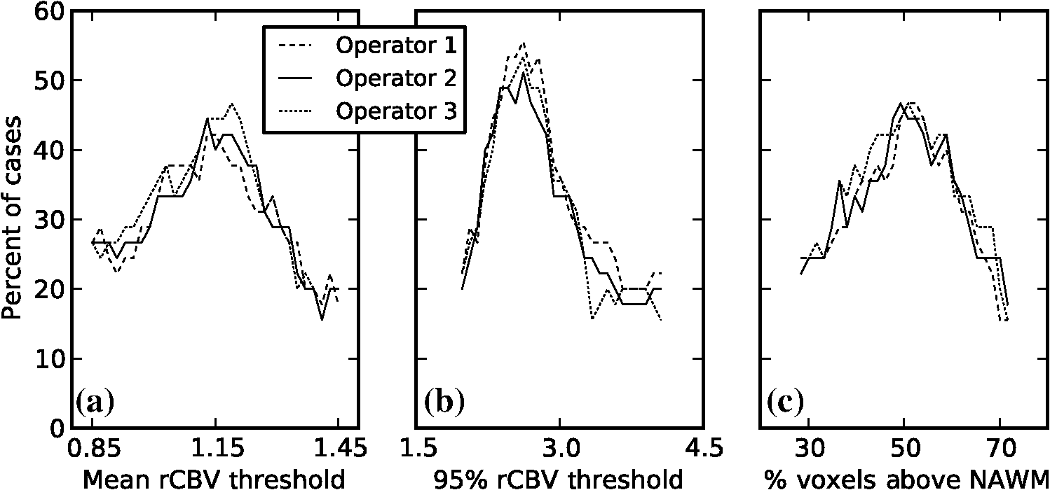

Fig. 6

Percentage of cases where one software package disagreed from other two (by software). Operator 1’s data. The $x$ axis range plotted is for all software’s percent of cases above the threshold (as shown in Fig. 4) being between 25% and 75%. The threshold is used to differentiate between pseudoprogression and progression. (a) The percentage of cases where one software package disagreed from the other two across a range of mean rCBV thresholds. (b) The percentage of cases where one software package disagreed from the other two across a range of 95th percentile rCBV thresholds. (c) The percentage of cases where one software package disagreed from the other two across a range of thresholds for percent of voxels above NAWM.

With the assumption that pseudoprogression may occur in roughly half of this cohort, the mean rCBV value at which IB Neuro splits the cases in half is $\sim 0.2$ below the value at which the other software split the cases in half. Alternatively, at a 95% rCBV threshold of 2.7, nordicICE classifies $\sim 50 %$ more cases as above the threshold (progressing tumor) than FuncTool. There is no single value where all three packages had reasonably high agreement, other than extreme values, where all cases would be considered progression or pseudoprogression.

For case-by-case analysis, Fig. 5 displays the percentage of cases where one software provides a different classification result than the other two, depending on the rCBV metric threshold used. Particular thresholds of interest would be based on the estimated incidence of progression versus pseudoprogression among the cases. The percentage of cases with disagreement ranges from the 20s to the 50s. The mean rCBV and % voxels above NAWM metrics have similar disagreement curves, with 95% rCBV peaking higher. The interoperator differences are small. Figure 6 displays the percentage of cases with discordant classification for each software package for a range of thresholds. This figure uses data from operator 1, as the small interoperator difference in Fig. 5 suggests it is representative of other operators. As expected from Fig. 4, IB Neuro disagrees more for mean rCBV, nordicICE disagrees more for 95% rCBV, and IB Neuro or FuncTool disagrees more for % voxels above NAWM.

3.2.

Outcome Prediction

The number of cases classified as progression or pseudoprogression using the three different criteria are shown in Table 3. More of the cases were classified as progression than pseudoprogression in the 1.5 T dataset, but less than half in the 3 T dataset. The area under the curve (AUC) measurements are shown in Table 4 for all the cases pooled together, with Table 5 displaying the results for the 1.5 and 3 T datasets analyzed separately. The 1.5 and 3 T pooled dataset showed poor performance of rCBV measures, with none of the instances having a 95% $CI > 0.5$ . However, the 3 T dataset had multiple instances where the AUC was significantly $> 0.5$ based on the 95% confidence interval. Additionally, despite the low numbers, the 3 T dataset had statistically significantly higher AUCs for the mean rCBV metric than the 1.5 T dataset. When nordicICE was used, the % voxels above NAWM metric also resulted in significantly higher AUCs for the 3 T group than the 1.5 T group. There was no statistically significant difference for any of the three metrics between the software or operators. Additionally, none of the three metrics performed better than the others.

Table 3

Number of images for each classification and magnet strength.

Magnet strength	Survival classification		Treatment change classification		Combined classification
Magnet strength	Prog	PsP	Prog	PsP	Prog	PsP
1.5 T	12	9	15	11	8	6
3 T	5	8	7	10	3	7
1.5 or 3 T	17	17	22	21	11	13

Note: Prog, progression; PsP, pseudoprogression.; Survival classification eliminated middle 20% of cases. Combined classification inclusion required agreement between the survival and treatment change classification methods.

Table 4

Area under the ROC curve for all 1.5 and 3 T images combined.

Operator	Software	Survival classification			Treatment change classification			Combined classification
Operator	Software	Mean rCBV	95% rCBV	% voxels above NAWM	Mean rCBV	95% rCBV	% voxels above NAWM	Mean rCBV	95% rCBV	% voxels above NAWM
1	IB Neuro	0.523	0.511	0.539	0.595	0.621	0.587	0.645	0.627	0.639
	FuncTool	0.503	0.523	0.516	0.582	0.578	0.584	0.590	0.603	0.615
	nordicICE	0.542	0.598	0.511	0.569	0.591	0.589	0.645	0.663	0.633
2	IB Neuro	0.523	0.511	0.539	0.595	0.621	0.587	0.645	0.627	0.639
	FuncTool	0.549	0.526	0.536	0.600	0.571	0.594	0.686	0.603	0.667
	nordicICE	0.542	0.588	0.529	0.565	0.579	0.577	0.627	0.633	0.639
3	IB Neuro	0.523	0.511	0.539	0.595	0.621	0.587	0.645	0.627	0.639
	FuncTool	0.513	0.516	0.529	0.576	0.573	0.598	0.635	0.641	0.647
	nordicICE	0.529	0.582	0.520	0.593	0.615	0.587	0.663	0.686	0.639

Note: All 95% CIs included 0.5.

Table 5

Area under the ROC curve for 1.5 and 3 T images separately.

Magnet strength	Op.	Software	Survival classification			Treatment change classification			Combined classification
Magnet strength	Op.	Software	Mean rCBV	95% rCBV	% voxels above NAWM	Mean rCBV	95% rCBV	% voxels above NAWM	Mean rCBV	95% rCBV	% voxels above NAWM
1.5 T	1	IB Neuro	0.437	0.484	0.452	0.583	0.701	0.561	0.500	0.650	0.483
		FuncTool	0.427	0.487	0.479	0.545	0.614	0.597	0.407	0.537	0.500
		nordicICE	0.484	0.571	0.460	0.508	0.540	0.561	0.517	0.600	0.483
	2	IB Neuro	0.437	0.484	0.452	0.583	0.701	0.561	0.500	0.650	0.483
		FuncTool	0.444	0.487	0.462	0.563	0.608	0.597	0.481	0.519	0.519
		nordicICE	0.508	0.587	0.500	0.524	0.540	0.578	0.500	0.600	0.517
	3	IB Neuro	0.437	0.484	0.452	0.583	0.701	0.561	0.500	0.650	0.483
		FuncTool	0.368	0.453	0.470	0.517	0.608	0.580	0.370	0.574	0.500
		nordicICE	0.468	0.595	0.468	0.567	0.626	0.578	0.517	0.683	0.483
3.0 T	1	IB Neuro	0.725	0.750	0.725	0.729	0.657	0.714	0.905a	0.905a	0.857a
		FuncTool	0.825a^,b	0.800a	0.750	0.843a	0.743a	0.686	1.000a^,b	0.952a^,b	0.857a
		nordicICE	0.800	0.775	0.750	0.843a	0.786	0.757	1.000a^,b	0.952a	0.952a^,b
	2	IB Neuro	0.725	0.750	0.725	0.729	0.657	0.714	0.905a	0.905a	0.857a
		FuncTool	0.800a	0.775	0.750	0.729	0.700	0.657	0.952a^,b	0.952a^,b	0.857a
		nordicICE	0.750	0.750	0.775	0.786a	0.757	0.800a	1.000a^,b	0.952a	1.000a^,b
	3	IB Neuro	0.725	0.750	0.725	0.729	0.657	0.714	0.905a	0.905a	0.857a
		FuncTool	0.800a^,b	0.800a^,b	0.675	0.757	0.671	0.657	0.952a^,b	0.952a	0.762
		nordicICE	0.750	0.750	0.775	0.800a	0.743	0.786a	1.000a^,b	0.952a	1.000a^,b

^aThe 95% CI is above 0.5.

^bThe 3 T value was statistically significantly higher (p<0.05) than the corresponding 1.5 T value, using the Delong method for comparison.; Op., operator.

The sensitivity and specificity analysis is shown in Tables 6 Table 7 through 8 for operator 1’s data. The optimal thresholds often differed between the software packages, and this resulted in differences in sensitivity and specificity that were statistically significant in many cases. The optimal threshold for the 3 T dataset was always higher than for the 1.5 T dataset, except FuncTool’s optimal thresholds for the % voxels above NAWM metric and the combined classification ground truth criterion. For the mean rCBV metric, the optimal threshold for 1.5 T ranged from 0.87 to 1.44, and that for 3.0 T from 1.10 to 1.52, depending on the software and classification criteria. For the 95% rCBV metric, the 1.5 T range was 2.0 to 3.04 and 3.0 T range was 2.64 to 4.00. The % voxels above NAWM metric produced optimal threshold ranges of 32.5 to 72.4 for 1.5 T (32.5 to 55.7 if the 72.4 threshold is removed), and 49.5 to 58.5 for 3.0 T.

Table 6

Sensitivity and specificity at optimal thresholds for each software and magnet strength. Metric: Mean rCBV.

Class. criteria	Software	1.5 T		3 T		1.5 T		3 T		1.5 T		3 T
		IB Neuro				FuncTool				nordicICE
		Thresh: 1.09		Thresh: 1.10		Thresh: 1.06		Thresh: 1.33		Thresh: 1.16		Thresh: 1.39
		Sens	Spec	Sens	Spec	Sens	Spec	Sens	Spec	Sens	Spec	Sens	Spec
Survival	IB Neuro	0.44	0.67a	0.80	0.63a	0.44b	0.56	0.40b	0.88	0.31b	0.67	0.40b	0.88
	FuncTool	0.60	0.44	1.00	0.38	0.60	0.44	0.80	0.75	0.47	0.44	0.60	0.75
	nordicICE	0.63	0.22a	0.80	0.25a	0.69b	0.22	0.80b	0.75	0.56b	0.44	0.80b	0.88
		Thresh: 0.87		Thresh: 1.41		Thresh: 0.98		Thresh: 1.39		Thresh: 1.13		Thresh: 1.50
		Sens	Spec	Sens	Spec	Sens	Spec	Sens	Spec	Sens	Spec	Sens	Spec
Treatment change	IB Neuro	0.79	0.55	0.57	0.90	0.53a^,b	0.55	0.57a^,b	0.90	0.26c^,d	0.64	0.43c^,d	1.00
	FuncTool	0.78	0.36	0.86	0.80	0.72b	0.45	0.86b	0.80	0.61c	0.45	0.57c	1.00
	nordicICE	0.89	0.27	0.71	0.90	0.84a	0.27	0.71a	0.80	0.68d	0.36	0.71d	1.00
		Thresh: 1.09		Thresh: 1.10		Thresh: 1.44		Thresh: 1.45		Thresh: 1.31		Thresh: 1.52
		Sens	Spec	Sens	Spec	Sens	Spec	Sens	Spec	Sens	Spec	Sens	Spec
Combined	IB Neuro	0.58	0.50	1.00	0.71	0.17	0.83	0.33	1.00	0.25	0.50	0.33	1.00
	FuncTool	0.82	0.17	1.00	0.43	0.36	0.67	1.00	0.86	0.45	0.33	0.67	1.00
	nordicICE	0.75	0.17	1.00	0.29	0.25	0.83	1.00	1.00	0.42	0.50	1.00	1.00

Note: Operator 1’s data. Comparison of sensitivity and specificity performed by pooling the 1.5 and 3 T cases of disagreement before calculating the test statistic.

^aComparison p value=0.016

^bComparison p value=0.031

^cComparison p value=0.046

^dComparison p value=0.0047

4. Discussion

DSC perfusion imaging is widely used in brain tumor imaging. In all cases, some form of postprocessing is required to convert the acquired images into a clinically relevant image, such as an rCBV image. The processing required to compute the rCBV includes identification of the time point where the bolus arrives and ends. The area under the relaxivity change curve created by this bolus is the basis of CBV determination. The challenge is that these images have a low signal-to-noise ratio (SNR), and contrast leakage can result in different baseline intensity after the bolus compared to before the bolus, and the baseline after the bolus can have a slope. Overall, the Boxerman et al.¹⁵ modeling method represents the most widely used and accepted model to date. Yet, which models the software programs implement can vary, and the specific method of implementation is often not readily available. IB Neuro and nordicICE employ the Boxerman model as the basis of their algorithm, while GE FuncTool uses linear interpolation from the prebolus and postbolus baselines when calculating the AUC.

Our study suggests that using different software packages results in clinically significant differences in CBV images, but using different operators produces just mild variability. It is important to note that the measurement comparisons we made were for the exact same voxels—the only variables were the software and the operator. While little operator variability was seen, substantial variation between software was seen. This variation was not something as simple as a scaling factor, which one could reasonably expect to see. The differences showed some patterns, with one software package being an outlier compared to the other two for each of the three metrics, but for each metric, a different package was the outlier. The variation is not based on the selection of any particular threshold, but for a broad range of threshold values, the clinical interpretation of the enhancing tissue would be different, depending only on the software used.

Normalization of rCBV values through the use of an NAWM mean appears insufficient as a postprocessing step to correct for variation. Normalization through removal of additive bias still did not increase the ICCs to over 0.9, and that is an optimistic correction that only works if the additive bias can be perfectly known on both an intersoftware and operator-specific basis. Regardless, a simple additive bias correction would have mostly empirical support rather than robust theoretical support.

One reassuring aspect of this study was the small variation between operators for a given software package. This suggests that if operators are given criteria for processing using a given software package, the results can be reproduced.

While previous papers published revealed differences in mean rCBV measurements from clinical images between software,¹⁷^,¹⁸ this work makes the additional contributions of analysis of the other previously published metrics of 95th % and % voxels above NAWM. While the other metrics did not prove to be more resistant to intersoftware variability, they had different, large effects on the intersoftware variability without eliminating it. Additional new contributions were that the software packages investigated were expanded to include IB Neuro, and interoperator differences were analyzed. Finally, the results were analyzed within a threshold-based framework, allowing for better estimation of the effect on clinical practice of the measurement differences.

The outcome-based GBM progression classification performance analysis using three different definitions of pseudoprogression did not detect a difference between the software when receiver operating characteristic curves (ROCs) were constructed with the software-specific threshold ranges. However, when an optimal threshold found for one software was used for the other software, there were many instances of statistically significant differences in sensitivity and specificity. Previously published optimal thresholds for determining tumor progression or recurrence have ranged from 0.71⁹ to 1.47¹¹ to 1.8¹⁰ to 2.6.⁸ However, the discrepancy could be attributed to differences in tumor types allowed in the studies, some allowing tumors other than GBM or high-grade gliomas, or differences in ROI approaches, with different numbers of hotspot voxels or entire tumors being used. It was unclear, though, how much of the difference could be due to the use of different software for CBV computation. For the survival classification criterion, 95% rCBV metric, and the 3 T images, this study’s optimal thresholds ranged from 2.64 to 3.19 to 3.50 depending on the software used, with all other variables fixed. For the mean rCBV metric, this study’s optimal thresholds were 1.10, 1.33, and 1.39 depending on the software package. While the ROI approach or rCBV metric used clearly has a significant effect on the optimal threshold values, the software effect itself is not negligible.

One note of caution is that, in general, the 3 T rCBV values were higher than the 1.5 T values despite the 3 T group having more pseudoprogression cases than progression. This observation is further confirmation of a study that imaged 21 patients at both 1.5 and 3 T and found that the 3 T rCBV was statistically significantly greater for the tumors ( $p = . 0041$ ).³⁰ While that study had differences in acquisition parameters besides field strength, our study confirms those findings with the magnet strength being the only variable. The superior performance of 3 T is likely due to the increased T1 and susceptibility weighting for 3 T versus 1.5 T. For this reason, 1.5 and 3 T data should not be pooled together for accuracy analysis since they likely have different optimal thresholds. For the cases in this study, the optimal thresholds shown in Tables 6 Table 7 through 8 were always higher for the 3 T dataset than the 1.5 T dataset, except for FuncTool’s thresholds for the combined-classification criterion using the % voxels above NAWM metric. This anomaly could be due to the lower combined-classification number of cases as well as the AUC being 0.500 for that combination of software, metric, and ground truth criterion.

Table 7

Sensitivity and specificity at optimal thresholds for each software and magnet strength. Metric: 95% rCBV.

Class. criteria	Software	1.5 T		3 T		1.5 T		3 T		1.5 T		3 T
		IB Neuro				FuncTool				nordicICE
		Thresh: 2.20		Thresh: 2.64		Thresh: 2.03		Thresh: 3.19		Thresh: 3.04		Thresh: 3.50
		Sens	Spec	Sens	Spec	Sens	Spec	Sens	Spec	Sens	Spec	Sens	Spec
Survival	IB Neuro	0.63	0.56a	1.00	0.63a	0.69	0.44	0.60	0.75	0.19a	0.89	0.20a	0.75
	FuncTool	0.53	0.56	0.80	0.50	0.67	0.56	0.80	0.75	0.07a	0.89	0.40a	1.00
	nordicICE	0.88	0.22a	0.80	0.13a	0.94	0.22	0.80	0.63	0.44a	0.44	0.80a	0.88
		Thresh: 2.25		Thresh: 3.41		Thresh: 2.00		Thresh: 3.31		Thresh: 2.78		Thresh: 3.50
		Sens	Spec	Sens	Spec	Sens	Spec	Sens	Spec	Sens	Spec	Sens	Spec
Treatment change	IB Neuro	0.68	0.73b	0.71	0.80b	0.84	0.45	0.71	0.80	0.32c	0.82b	0.43c	0.80b
	FuncTool	0.44c	0.55	0.57c	0.80	0.72b	0.45	0.57b	0.80	0.06d	0.91a	0.43d	0.80a
	nordicICE	0.95c	0.36b	0.71c	0.60b	1.00b	0.27	0.71b	0.60	0.74c^,d	0.45a^,b	0.71c^,d	0.60a^,b
		Thresh: 2.20		Thresh: 3.41		Thresh: 2.54		Thresh: 3.31		Thresh: 2.94		Thresh: 4.00
		Sens	Spec	Sens	Spec	Sens	Spec	Sens	Spec	Sens	Spec	Sens	Spec
Combined	IB Neuro	0.75	0.67	1.00	0.86	0.33a	0.67	1.00a	0.86	0.25	0.83	0.33	0.86
	FuncTool	0.73	0.33	0.67	0.86	0.45b	0.83	0.67b	0.86	0.09	0.83	0.67	1.00
	nordicICE	1.00	0.33	1.00	0.72	0.92a^,b	0.33	1.00a	0.71	0.50	0.50	1.00	0.86

Note: Operator 1’s data. Comparison of sensitivity and specificity performed by pooling the 1.5 and 3 T cases of disagreement before calculating the test statistic.

^aComparison p value=0.016

^bComparison p value=0.031

^cComparison p value=0.0047

^dComparison p value=0.00053

Table 8

Sensitivity and specificity at optimal thresholds for each software and magnet strength. Metric: % above NAWM.

Class. criteria	Software	1.5 T		3 T		1.5 T		3 T		1.5 T		3 T
		IB Neuro				FuncTool				nordicICE
		Thresh: 32.5		Thresh: 50		Thresh: 55.7		Thresh: 58.0		Thresh: 42.6		Thresh: 49.6
		Sens	Spec	Sens	Spec	Sens	Spec	Sens	Spec	Sens	Spec	Sens	Spec
Survival	IB Neuro	0.63	0.56	0.60	0.88	0.31a	0.67	0.00a	0.88	0.44b	0.56	0.60b	0.88
	FuncTool	0.67	0.33	1.00	0.50	0.47a	0.44	0.80a	0.63	0.67b	0.44	1.00b	0.50
	nordicICE	0.75	0.22	0.60	0.75	0.25a	0.78	0.20a	0.88	0.56	0.56	0.60	0.75
		Thresh: 32.5		Thresh: 54.2		Thresh: 38.6		Thresh: 56.8		Thresh: 35.0		Thresh: 49.5
		Sens	Spec	Sens	Spec	Sens	Spec	Sens	Spec	Sens	Spec	Sens	Spec
Treatment change	IB Neuro	0.68	0.55	0.57	1.00	0.47c	0.55	0.58c	0.55	0.58b	0.55	0.57b	0.90
	FuncTool	0.83	0.45	0.86	0.60	0.78c	0.45	0.83c	0.45	0.83b	0.45	0.86b	0.40
	nordicICE	0.89	0.45	0.29	1.00	0.68	0.45	0.84	0.45	0.84	0.45	0.57	0.80
		Thresh: 32.5		Thresh: 55.6		Thresh: 72.4		Thresh: 58.5		Thresh: 44.1		Thresh: 49.7
		Sens	Spec	Sens	Spec	Sens	Spec	Sens	Spec	Sens	Spec	Sens	Spec
Combined	IB Neuro	0.83	0.33	0.67	1.00	0.17b	1.00	0.00b	1.00	0.50	0.33	0.67	1.00
	FuncTool	0.91	0.17	1.00	0.71	0.45b	0.67	0.67b	0.71	0.82	0.17	1.00	0.57
	nordicICE	1.00	0.17	0.33	1.00	0.17	1.00	0.33	1.00	0.75	0.33	0.67	0.86

Note: Operator 1’s data. Comparison of sensitivity and specificity performed by pooling the 1.5 and 3 T cases of disagreement before calculating the test statistic.

^aComparison p value=0.016

^bComparison p value=0.031

^cComparison p value=0.0078

These data support the use of 3 T DSC-MR imaging of GBM patients as opposed to 1.5 T imaging for distinguishing tumor progression or pseudoprogression with spin-echo acquisitions using similar preload dosing. While the same patients were not imaged at both 1.5 and 3 T for direct comparison, and the numbers were small for 3 T, statistical significance was found for the 3 T performance advantage. Due to the importance of this finding, further investigation with larger numbers of cases is indicated.

The lack of statistical significance in AUC differences between software could be reflective of inadequacy of the survival- and treatment-based classification criteria, or the number of cases. Additionally, the analysis can be susceptible to small differences in treatment. Since intermediate survival cases were excluded, the ROC curves using the survival criterion are optimistic. However, as days survived is a surrogate marker for another characteristic that is continuous in reality, progression, the potential bias effect is somewhat muted. The combined-classification criterion similarly has the potential to produce a higher performance estimate than would occur in analysis of new, unknown cases due to the excluded cases. However, it also could be considered the stronger, more accurate classification method than the other two separately since it eliminates cases with a more uncertain classification from the analysis.

A common practice on the use of rCBV values, as described in other papers, is for users to select ROIs using the rCBV images. That practice is suboptimal because it introduces dependency on the user and makes the method challenging to reproduce. Because it is not matched to areas of enhancement, it also is unclear what the hotspots represent on conventional imaging. Nevertheless, the point of this paper is that the actual rCBV values that one would see on an rCBV image will depend heavily on the software used.

There is strong interest in promoting the use of quantitative imaging, but the results here suggest that how rCBV is calculated must be more thoroughly examined before quantitation can be broadly applied. Either some correction factor will need to be found for each software/rCBV metric, an approach not likely successful based on this study’s data, or the studies published for a given software and CBV metric will need to be reproduced with the other software and metric methods to determine the proper thresholds. We note here that the three packages included in our study represent the vast majority of publications that use FDA-cleared software. Because these are proprietary commercial packages, certain details of the algorithm are not available, making it difficult to understand, characterize, or correct for the differences. While there is an accepted general model of the effect of gadolinium on DSC images, specifics of how the baselines before and after the bolus are determined, how leakage rates after the bolus are determined, assumptions about how to correct for the observed leakage, and noise estimation methods are all critical to computing the rCBV, but unless vendors share their specific algorithms, it will be difficult to explain the basis for the differences we found.

It should be noted that the analyzed images were spin-echo echo-planar T2W acquisitions, and similar results may not occur with gradient recalled echo acquisitions or spin-echo acquisitions using different contrast administration protocols. However, a decrease in variability was not seen when the 3 T acquired data were compared with the 1.5 T acquired data (see Table 9), suggesting precise acquisition methods or signal-to-noise are not significant factors. Further studies are needed to evaluate postprocessing differences using gradient recalled echo data. Some have suggested that spin-echo acquisitions may be more appropriate for brain tumors because it emphasizes the smaller vessels seen in brain tumors, compared to the large vessel occlusions seen in vascular disease. While this is a theoretical advantage, we are not aware of a study documenting an advantage, and this question warrants further study. Regarding other aspects of the acquisition protocols, this was a retrospective study and their parameters could not be altered since they were the clinical protocols used. Increased matrix size might possibly increase the software divergence due to increased noise, but lower magnetic strength (with lower SNR) did not show increased divergence. Regarding increasing the temporal resolution, we did look to see whether there was a noticeable difference in variability when the cases were limited to those with subjectively better bolus curves, and did not find any. However, better temporal resolution might indeed decrease the variability. The same NAWM and tumor ROIs were used across operator and software, so sampling effects should not have influenced the measured variability.

Table 9

Intersoftware ICC—operator 1’s data.

Magnet strength	Metric	ICC (95% CI)
Magnet strength	Metric	Agreement	Consistency
1.5 T	Mean rCBV	0.851 (0.690, 0.930)	0.889 (0.807, 0.942)
	95% rCBV	0.611 (0.172, 0.827)	0.798 (0.664, 0.891)
	% voxels above NAWM	0.737 (0.422, 0.881)	0.833 (0.717, 0.911)
3.0 T	Mean rCBV	0.651 (0.371, 0.847)	0.701 (0.453, 0.871)
	95% rCBV	0.707 (0.393, 0.882)	0.787 (0.585, 0.911)
	% voxels above NAWM	0.487 (0.095, 0.774)	0.680 (0.422, 0.860)

Note: Agreement: Comparison of raw values; Consistency: Comparison of values with software-specific means subtracted.

In this study, the ROI used is only the enhancing component of the image. It is well-known that the region of enhancement does not represent the true extent of infiltrating glioma. Therefore, while the ROI for this study may not be entirely representative, it is exactly the enhancing component that requires differentiation of progression versus pseudoprogression. Because the software is proprietary, we do not have access to the model used to estimate and correct for leakage, but this is likely one source of variability between the software packages. Detecting progression in areas of nonenhancement is clearly an important concern and could ultimately yield intersoftware performance differences in future studies. However, the regions of enhancement are presumed to provide the most intersoftware differences due to the leakage correction variable. Similarly, lower-grade gliomas would be expected to have decreased rCBV variability due to decreased leakage, although this needs to be confirmed in future studies.

Limiting our patient cohort to GBM patients treated with radiation and temozolomide represents a select group. However, this treatment regimen is quite common and is associated with frequent occurrences of MRI changes for which perfusion is selected as an important characteristic to interpret. Use of anti-angiogenic agents will substantially alter the perfusion and enhancement characteristics, and while used commonly in this patient group, this very different clinical situation would potentially confound our findings rather than improve it, and deserves separate attention.

rCBV values were found to be useful for distinguishing GBM progression from pseudoprogression, as previously shown in the literature. However, as one specific software package or rCBV metric did not provide more useful information than the others, we cannot recommend a specific software package for use in multicenter studies based on these study results. Further studies are needed to evaluate DSC data acquired through other methods (such as gradient recalled echo). It is critical, though, that individual trials use the same software package and same DSC acquisition methods to generate each patient’s rCBV images. Additionally, these data show that acquiring images at 3.0 T produces both different optimal thresholds and more valuable information for determining GBM progression than 1.5 T for spin-echo acquisitions.

As more research is conducted regarding the use of rCBV, clinicians are relying upon it more frequently for help with diagnosis and treatment planning. Consequently, accuracy and precision of rCBV measurements become increasingly important as the analysis becomes more quantitative. This study’s implication for clinical practice is clear: care must be taken to assure that if thresholds are used in clinical practice that are based on the literature, the same software and processing methods must be applied. Additionally, when comparing exams for the same patient or pooling exams for an rCBV study, the same CBV calculation software should be used. This report raises serious doubt about the ability to use quantitative rCBV measures without requiring a specific, consistent software for processing.

Acknowledgments

We wish to acknowledge the support of NIH (1U01CA160045-01A1) and the Mayo Medical Scientist Training Program. We wish to thank Mandie Maroney-Smith for her assistance with image processing.

References

1.

S. A. Grossman et al., “Survival of patients with newly diagnosed glioblastoma treated with radiation and temozolomide in research studies in the United States,” Clin. Cancer Res., 16 (8), 2443 –2449 (2010). http://dx.doi.org/10.1158/1078-0432.CCR-09-3106 CCREF4 1078-0432 Google Scholar

2.

R. Stupp et al., “Effects of radiotherapy with concomitant and adjuvant temozolomide versus radiotherapy alone on survival in glioblastoma in a randomised phase III study: 5-year analysis of the EORTC-NCIC trial,” Lancet Oncol., 10 (5), 459 –466 (2009). http://dx.doi.org/10.1016/S1470-2045(09)70025-7 LOANBN 1470-2045 Google Scholar

3.

M. C. Y. de Wit et al., “Immediate post-radiotherapy changes in malignant glioma can mimic tumor progression,” Neurology, 63 (3), 535 –537 (2004). http://dx.doi.org/10.1212/01.WNL.0000133398.11870.9A NEURAI 0028-3878 Google Scholar

4.

J. L. Clarke and S. Chang, “Pseudoprogression and pseudoresponse: challenges in brain tumor imaging,” Curr. Neurol. Neurosci. Rep., 9 (3), 241 –246 (2009). http://dx.doi.org/10.1007/s11910-009-0035-4 CNNRBS 1528-4042 Google Scholar

5.

E. Topkan et al., “Pseudoprogression in patients with glioblastoma multiforme after concurrent radiotherapy and temozolomide,” Am. J. Clin. Oncol., 35 (3), 284 –289 (2012). http://dx.doi.org/10.1097/COC.0b013e318210f54a AJCODI 0277-3732 Google Scholar

6.

R. J. Young et al., “Potential utility of conventional MRI signs in diagnosing pseudoprogression in glioblastoma,” Neurology, 76 (22), 1918 –1924 (2011). http://dx.doi.org/10.1212/WNL.0b013e31821d74e7 NEURAI 0028-3878 Google Scholar

7.

J. M. Provenzale, S. Mukundan and D. P. Barboriak, “Diffusion-weighted and perfusion MR imaging for brain tumor characterization and assessment of treatment response,” Radiology, 239 (3), 632 –649 (2006). http://dx.doi.org/10.1148/radiol.2393042031 RADLAX 0033-8419 Google Scholar

8.

T. Sugahara et al., “Posttherapeutic intraaxial brain tumor: the value of perfusion-sensitive contrast-enhanced MR imaging for differentiating tumor recurrence from nonneoplastic contrast-enhancing tissue,” Am. J. Neuroradiol., 21 (5), 901 –909 (2000). 0195-6108 Google Scholar

9.

L. S. Hu et al., “Relative cerebral blood volume values to differentiate high-grade glioma recurrence from posttreatment radiation effect: direct correlation between image-guided tissue histopathology and localized dynamic susceptibility-weighted contrast-enhanced perfusion MR imaging measurements,” Am. J. Neuroradiol., 30 (3), 552 –558 (2009). http://dx.doi.org/10.3174/ajnr.A1377 0195-6108 Google Scholar

10.

E. L. Gasparetto et al., “Posttreatment recurrence of malignant brain neoplasm: accuracy of relative cerebral blood volume fraction in discriminating low from high malignant histologic volume fraction,” Radiology, 250 (3), 887 –896 (2009). http://dx.doi.org/10.1148/radiol.2502071444 RADLAX 0033-8419 Google Scholar

11.

D. S. Kong et al., “Diagnostic dilemma of pseudoprogression in the treatment of newly diagnosed glioblastomas: the role of assessing relative cerebral blood flow volume and oxygen-6-methylguanine-DNA methyltransferase promoter methylation status,” Am. J. Neuroradiol., 32 (2), 382 –387 (2011). http://dx.doi.org/10.3174/ajnr.A2286 0195-6108 Google Scholar

12.

E. S. Paulson and K. M. Schmainda, “Comparison of dynamic susceptibility-weighted contrast-enhanced MR methods: recommendations for measuring relative cerebral blood volume in brain tumors,” Radiology, 249 (2), 601 –613 (2008). http://dx.doi.org/10.1148/radiol.2492071659 RADLAX 0033-8419 Google Scholar

13.

J. L. Boxerman et al., “The role of preload and leakage correction in gadolinium-based cerebral blood volume estimation determined by comparison with MION as a criterion standard,” Am. J. Neuroradiol., 33 (6), 1081 –1087 (2012). http://dx.doi.org/10.3174/ajnr.A2934 0195-6108 Google Scholar

14.

M. Law et al., “Comparison of cerebral blood volume and vascular permeability from dynamic susceptibility contrast-enhanced perfusion MR imaging with glioma grade,” Am. J. Neuroradiol., 25 (5), 746 –755 (2004). 0195-6108 Google Scholar

15.

J. L. Boxerman, K. M. Schmainda and R. M. Weisskoff, “Relative cerebral blood volume maps corrected for contrast agent extravasation significantly correlate with glioma tumor grade, whereas uncorrected maps do not,” AJNR Am. J. Neuroradiol., 27 (4), 859 –867 (2006). 0195-6108 Google Scholar

16.

K. Kudo et al., “Accuracy and reliability assessment of CT and MR perfusion analysis software using a digital phantom,” Radiology, 267 (1), 201 –211 (2013). http://dx.doi.org/10.1148/radiol.12112618 RADLAX 0033-8419 Google Scholar

17.

L. Orsingher, S. Piccinini and G. Crisi, “Differences in dynamic susceptibility contrast MR perfusion maps generated by different methods implemented in commercial software,” J. Comput. Assist. Tomogr., (2014). http://dx.doi.org/10.1097/RCT.0000000000000115 JCATD5 0363-8715 Google Scholar

18.

M. V. Milchenko et al., “Comparison of perfusion- and diffusion-weighted imaging parameters in brain tumor studies processed using different software platforms,” Acad. Radiol., (2014). http://dx.doi.org/10.1016/j.acra.2014.05.016 1076-6332 Google Scholar

19.

P. A. Yushkevich et al., “User-guided 3D active contour segmentation of anatomical structures: significantly improved efficiency and reliability,” NeuroImage, 31 (3), 1116 –1128 (2006). http://dx.doi.org/10.1016/j.neuroimage.2006.01.015 NEIMEF 1053-8119 Google Scholar

20.

N. Otsu, “A threshold selection method from gray-level histograms,” IEEE Trans. Syst. Man Cybern., 9 (1), 62 –66 (1979). http://dx.doi.org/10.1109/TSMC.1979.4310076 ITSHFX 1083-4427 Google Scholar

21.

M. Jenkinson et al., “FSL,” NeuroImage, 62 (2), 782 –790 (2012). http://dx.doi.org/10.1016/j.neuroimage.2011.09.015 NEIMEF 1053-8119 Google Scholar

22.

M. Jenkinson et al., “Improved optimization for the robust and accurate linear registration and motion correction of brain images,” NeuroImage, 17 (2), 825 –841 (2002). NEIMEF 1053-8119 Google Scholar

23.

S. M. Smith, “Fast robust automated brain extraction,” Hum. Brain Mapp., 17 (3), 143 –155 (2002). http://dx.doi.org/10.1002/(ISSN)1097-0193 HBRME7 1065-9471 Google Scholar

24.

L. S. Hu et al., “Reevaluating the imaging definition of tumor progression: perfusion MRI quantifies recurrent glioblastoma tumor fraction, pseudoprogression, and radiation necrosis to predict survival,” Neuro-Oncology, 14 (7), 919 –930 (2012). http://dx.doi.org/10.1093/neuonc/nos112 1522-8517 Google Scholar

25.

H. Kim et al., “Gliomas: application of cumulative histogram analysis of normalized cerebral blood volume on 3 T MRI to tumor grading,” PLoS ONE, 8 (5), e63462 (2013). http://dx.doi.org/10.1371/journal.pone.0063462 1932-6203 Google Scholar

26.

M. Gamer et al., “IRR: various coefficients of interrater reliability and agreement,” (2015) http://cran.r-project.org/web/packages/irr/ April ). 2015). Google Scholar

27.

R Core Team, “R: a language and environment for statistical computing,” (2015) http://web.mit.edu/r_v3.0.1/fullrefman.pdf April ). 2015). Google Scholar

28.

K. O. McGraw and S. P. Wong, “Forming inferences about some intraclass correlation coefficients,” Psychol. Methods, 1 (1), 30 (1996). http://dx.doi.org/10.1037/1082-989X.1.1.30 1082-989X Google Scholar

29.

E. Yaman et al., “Radiation induced early necrosis in patients with malignant gliomas receiving temozolomide,” Clin. Neurol. Neurosurg., 112 (8), 662 –667 (2010). http://dx.doi.org/10.1016/j.clineuro.2010.05.003 CNNSBV 0303-8467 Google Scholar

30.

N. Mauz et al., “Perfusion magnetic resonance imaging: comparison of semiologic characteristics in first-pass perfusion of brain tumors at 1.5 and 3 Tesla,” J. Neuroradiol., 39 (5), 308 –316 (2012). http://dx.doi.org/10.1016/j.neurad.2011.12.004 JNEUD3 Google Scholar

Biography

Zachary S. Kelm is an MD/PhD student at the Mayo Clinic in Rochester, Minnesota. He received his bachelor’s degree in mechanical engineering from Baylor University in 2006. He will complete his MD degree and biomedical engineering PhD degree training in 2015, with plans to train in a radiology residency. His research interests include medical image processing, image-based biomarkers, and computer-aided diagnosis.

Panagiotis D. Korfiatis is a senior research fellow at the Radiology Department of the Mayo Clinic. He received his BSc degree in physics, and MSc and PhD degrees in medical physics from the University of Patras, Patras, Greece, in 2004, 2006, and 2010, respectively. He is the author/coauthor of more than 13 journal papers. His current research interests include three-dimensional image analysis techniques, pattern recognition, and computer-aided diagnosis methods.

Ravi K. Lingineni received his MPH degree in biostatistics from the University of North Texas Health Science Center in 2012. He has been working as a biostatistician at the Mayo Clinic in Rochester since 2012. He is a coauthor of 18 peer-reviewed publications.

John R. Daniels is an MRI technologist at the Mayo Clinic in Scottsdale, Arizona. He received his associate of applied science: radiologic technology degree in 1991, followed by a bachelor’s degree in business administration in 2012. He was inducted into the Delta Mu Delta International Honor Society in 2012. He has worked at the Mayo Clinic within MR imaging since 2007, with special interests and/or training in MRI environment safety, quality control, scanning, protocols, and postprocessing.

Jan C. Buckner is a professor of oncology at the Mayo Clinic in Rochester, Minnesota. He obtained his MD degree from the University of North Carolina, Chapel Hill, in 1980, followed by internal medicine residency at Butterworth Hospital and a medical oncology fellowship at Mayo Clinic. He currently serves as the chair of the Department of Oncology. His research interests include studying the clinical significance of histologic and genetic variables in brain tumor tissue as well as methodologic issues in designing clinical trials for brain tumor patients.

Daniel H. Lachance is an associate professor of neurology at the Mayo Clinic in Rochester, Minnesota. He obtained his MD degree at Dartmouth Medical School in 1984, followed by neurology residency training at the Mayo Clinic and neuro-oncology fellowship training at Duke University. He currently serves as division chair for neuro-oncology at the Mayo Clinic in Rochester and has particular research interests in neuroimmunology, clinical neuro-oncology, and the genetic epidemiology of glioma.

Ian F. Parney is a neurosurgeon at the Mayo Clinic in Rochester, Minnesota. He received his MD degree in 1993 and PhD in 1999, both from the University of Alberta, where he also completed his neurosurgical residency in 2001. He received further subspecialty training in neuro-oncology at the University of California, San Francisco. His clinical and research interests are focused on adult malignant brain tumors. He has particular interests in intraoperative MRI, glioma immunology and immunotherapy, and clinical trials in neurosurgical oncology.

Rickey E. Carter is an associate professor of biostatistics in the Department of Health Sciences Research at the Mayo Clinic. He has a PhD in biostatistics from the Medical University of South Carolina. His current research interests are in the design and analysis of translational studies, integration of consumer and medical sensor technology into health, and design considerations for human observer performance studies. He is the author of over 160 journal articles and two book chapters.

Bradley J. Erickson received his MD and PhD degrees from the Mayo Clinic. He then trained in radiology and neuroradiology at Mayo, and has now practiced clinical neuroradiology there for more than 20 years. He has chaired the Radiology Informatics Division and is associate chair for research. He has been awarded multiple external grants, including NIH grants on MS, brain tumors, and medical image processing. His particular focuses are on the use of image processing and machine learning to improve understanding and the ability to diagnose these diseases.

CC BY: © The Authors. Published by SPIE under a Creative Commons Attribution 4.0 Unported License. Distribution or reproduction of this work in whole or in part requires full attribution of the original publication, including its DOI.

Citation Download Citation

Zachary S. Kelm, Panagiotis D. Korfiatis, Ravi K. Lingineni, John R. Daniels, Jan C. Buckner, Daniel H. Lachance, Ian F. Parney, Rickey E. Carter, and Bradley J. Erickson "Variability and accuracy of different software packages for dynamic susceptibility contrast magnetic resonance imaging for distinguishing glioblastoma progression from pseudoprogression," Journal of Medical Imaging 2(2), 026001 (26 May 2015). https://doi.org/10.1117/1.JMI.2.2.026001

Published: 26 May 2015

Access the abstract

JOURNAL ARTICLE
14 PAGES

DOWNLOAD PAPER SAVE TO MY LIBRARY

GET CITATION

CITATIONS

Cited by 25 scholarly publications.

Explore citations on Lens.org

KEYWORDS

Tumors

Magnetic resonance imaging

Brain

Image classification

Blood

Image segmentation

Tissues

1.

Introduction

Fig. 1

2.

Materials and Methods

2.1.

Patients

2.2.

MR Images

2.3.

DSC-MRI Processing

2.4.

Registration and Tumor Segmentation

Fig. 2

2.5.

rCBV Metrics

2.6.

rCBV Values

2.7.

Outcome Prediction

3.

Results

3.1.

rCBV Values

Table 1

Table 2

Fig. 3

Fig. 4

Fig. 5

Fig. 6

3.2.

Outcome Prediction

Table 3

Table 4

Table 5

Table 6

4.

Discussion

Table 7

Table 8

Table 9

Acknowledgments

References

Biography

Show All Keywords

Keywords/Phrases

Search In:

Publication Years