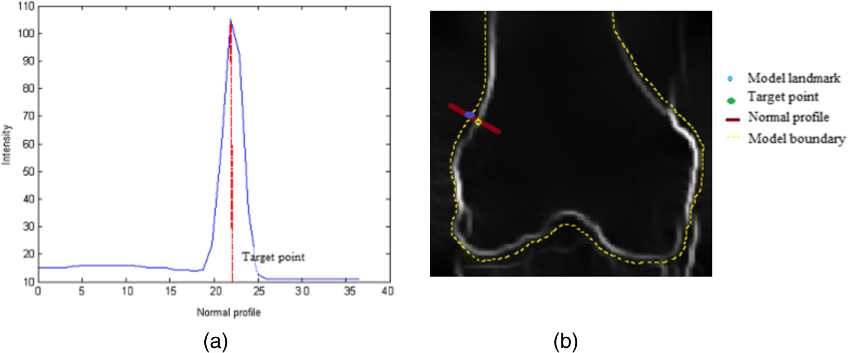
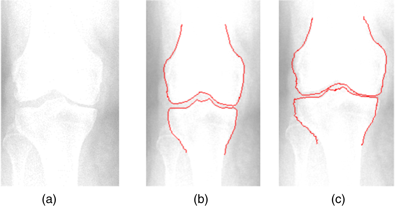
1.

Introduction

The segmentation of knee x-ray images has found wide applications in the analysis of anatomical structure and kinematics,^1–4 the assessment of loss of joint space width (JSW), the diagnosis of osteoarthritis (OA) and osteoporosis in terms of fracture detection and bone density measurement, and the planning for joint replacement.⁵ Manual segmentation of these anatomical structures is time consuming and subjective. Our aim is to design a robust automatic segmentation method to extract the distal femur and proximal tibia contours from x-ray images. However, automatic segmentation is challenging due to the complex structure of the knee in x-ray images. Images may be contaminated by noise, sampling artifacts, spatial aliasing, insufficient contrast or resolution, or luminous intensities depending on the x-ray equipment such that the boundaries of the regions of interest become indistinct or disconnected. Interpatient bone shape, size, and deformation variations, such as osteophytes, add complexity to structure identification. Moreover, the loss of key features of the femur contour may occur from overlapping neighboring bones, such as the tibia, and occlusion by implants or operational tools.

Previous work on automatic femur and tibia segmentation has primarily focused on using the active shape model (ASM).^6–9 ASM was first developed in the mid-1990s by Cootes et al.¹⁰ performing principal component analysis (PCA) on a series of manually marked training data to generate a statistical shape model. There are several advantages in using ASM: ASM has good performance for low contrast images and is based on user-defined forces. In addition, ASM is guided by prior knowledge of shape from manually annotated training dataset, making it less susceptible to imaging artifacts. Historically, the ASM has been modified and improved. Behiels et al.⁶ added a regulation term in the cost function to impose smoothness of shape changes. Lindner et al.⁷ integrated random forest regression voting to ASM to segment proximal femur. Seise et al.⁹ used a double contour active shape model to segment tibia and femur from knee x-ray images.

Original ASM using Mahalanobis distance (MD) to find the object of interest has some limitations. MD¹¹ is a statistical measurement to determine similarity between sets that are assumed to have normal distribution. In an x-ray image, the point with the minimum MD between its surrounding intensity values and the mean lies on the border of the object. The MD calculation involves the inverse of a covariance matrix of the training data. If the covariance matrix is sparse, its inverse will be undefined and consequently, MD will be undefined. The covariance matrix becomes sparse when the number of pixels sampled is greater than the number of training images. Therefore, either having a limited training dataset or attempting to sample a large number of pixels would prove problematic.

The active appearance model (AAM)¹² is another segmentation method that assumes the appearance spaces to be Gaussian. However, this assumption fails in real patients as the interpatient bone structure varies significantly, especially for bones with osteophytes. In such cases, a single mean mode is insufficient to capture the variations of appearance spaces with a single Gaussian distribution. A further limitation of AAM is that x-ray images of degenerated bones create outliers, which may lead to incorrect segmentation.

We present a robust segmentation method integrating spectral clustering and ASM to accurately extract bone contours in knee radiographs. Spectral clustering¹³ is an unsupervised learning algorithm to extract global information from an image so that only the most salient edge points remain and the original image has been denoised. Active contour search is then performed on the denoised x-ray image to obtain the candidate contour points with the highest intensity gradient. ASM constrains the contour in feasible shapes, leading to an accurate and robust segmentation result. This method captures large appearance variation, thus solving the limitations of ASM using MD and AAM.

The remainder of the paper is organized as follows: Sec. 2 provides a description of the segmentation framework, followed by the experiments and evaluation in Sec. 3 and conclusions in Sec. 4.

2.

Approach

The proposed method consists of two parts: spectral clustering for image denoising and ASM for segmentation. In the following section, we will discuss spectral clustering in Sec. 2.1, ASM in Sec. 2.2, and the overall segmentation algorithm in Sec. 2.3.

2.1.

Spectral Clustering

The traditional AAM¹² is constructed from the intensity distribution of the region of interest. However, the intensities of the femur and tibia in x-ray images may vary significantly with different equipment and intensity settings, leading to an inaccurate appearance model. For images with large, interdataset intensity variations, spectral clustering was employed to determine the similarity between image pixels in a similar manner to the “normalized cuts” approach by Shi and Malik.¹³ Spectral clustering relies on the eigenvalues and eigenvectors of an affinity matrix defined in Eq. (1) to partition points into disjoint clusters with high intracluster similarity and high intercluster dissimilarity. The eigenvectors obtained from spectral partitioning are then used as weighted candidates for the following oriented segmentation to create a direct partition of the image, rather than using a clustering algorithm, such as $k$-means clustering.¹³ Our method differs from the method of Shi and Malik in that eigenvectors obtained from spectral partitioning are treated as denoised images for the following ASM-based segmentation, rather than being directly partitioned by $k$-means clustering.

As an input to spectral clustering, a sparse symmetric affinity matrix $W$ is constructed using the intervening contour cue,¹⁴ which is the maximal value of intensity (Im) along a line connecting two pixels in the image. The two pixels have a low affinity as a strong boundary separates them from a high affinity in the same region. The affinity matrix is formed by connecting all pixels $i$ and $j$ within a fixed radius $r$ with affinity:

Eq. (1)

$$W_{ij}=\exp (-\underset{p\in \overline{ij}}{\max }\{\mathrm{Im}(p)/\rho \}),$$

where $\overline{ij}$ is the line segment connecting $i$ and $j$ and $\rho$ is a constant.

Shi and Malik¹³ proposed a normalized cut, $N\mathit{cut}(A,B)$, to describe the degree of dissimilarity between two sets, $A$ and $B$. The normalized cut can be minimized using the condition:

$$v(i)\in \{1,-\frac{{\sum }_{x_i>0}{d}_i}{{\sum }_{x_i<0}{d}_i}\}\text{and}{\mathrm{v}}^{\mathrm{T}}\mathrm{D}\mathbf{1}=0,\text{where}v=(1+x)-\frac{{\sum }_{x_i>0}{d}_i}{{\sum }_{x_i<0}{d}_i}(1-x)$$

to identify and delete the weakest link among nodes in a graph as follows:

Eq. (2)

$${\min }_{x}N\mathit{cut}(x)={\min }_v\frac{v^T(D-W)v}{v^{T}Dv},$$

where $D_{ij}={\mathrm{\Sigma }}_j{W}_{ij}$ is an element of $D$ in the $i$’th row and $j$’th column, and $x$ to be an $N=|V|$ dimensional indicator vector ($x_i=1$ if $x_i\in A$ and $x_i=-1$ otherwise).

Equation (2) is the Rayleigh quotient,¹⁵ which can be minimized by solving the generalized eigenvalue problem (generalized SVD):

Eq. (3)

$$(\mathbf{D}-\mathbf{W})\mathbf{v}=\lambda \mathbf{Dv},$$

where $D_{ij}={\mathrm{\Sigma }}_j{W}_{ij}$, $\{{\mathbf{v}}_0,{\mathbf{v}}_1,\dots ,{\mathbf{v}}_n\}$ is solved as generalized eigenvectors corresponding to the $n+1$ smallest eigenvalues $0={\lambda }_0\le {\lambda }_1\le \dots \le {\lambda }_n$. These generalized eigenvectors $\{{\mathbf{v}}_0,{\mathbf{v}}_1,\dots ,{\mathbf{v}}_n\}$ carry contour information¹⁶ themselves. Thus, each eigenvector, ${\mathbf{v}}_i$, is treated as an image, which is then filtered with Gaussian directional derivative filters at multiple orientations and weighted by ${\lambda }_i$ in Eq. (4):

Eq. (4)

$$\mathrm{SIm}(x,y)=\underset{\theta }{\max }[{\mathrm{\Sigma }}_i{\nabla }_{\theta }{v}_i(x,y)].$$

Equation (4) is maximized over the angle of the Gaussian directional derivative filter. The weighting by the eigenvalue ${\lambda }_i$ is motivated by the physical interpretation of the generalized eigenvalue problem as a mass-spring system.¹⁷

To demonstrate the spectral clustering’s ability to denoise the original x-ray image, the first seven generalized eigenvectors are depicted compared to the same image filtered by a $3\times 3$ Sobel operator,¹⁸ as shown in Fig. 1. In practice, 16 eigenvectors were used for spectral clustering.¹⁶ To qualitatively compare the results from spectral clustering and Sobel operator, the intensity of both images is normalized to [0,1], as shown in Figs. 1(i) and 1(j). Furthermore, we compared the signal-to-noise ratio (SNR) of these two images; SNR is 16.05 for the spectral clustering image in Fig. 1(i) and 10.04 for the Sobel filtered image in Fig. 1(j). Both qualitative and quantitative results show that spectral clustering outperforms the conventional Sobel operator, because it extracts only the most salient edges in the image while the latter extracts data at all the edges.

Fig. 1

X-ray image after spectral clustering and Sobel operator: (a) original image; (b)–(h) first seven generalized eigenvectors from spectral clustering; (i) output from spectral clustering; (j) Sobel filtered image. The intensity of both spectral clustering and Sobel operator images are normalized to [0,1].

2.2.

Active Shape Model

Two commonly used segmentation strategies after performing spectral clustering are k-way segmentation¹³ and hierarchical segmentation.¹⁶ K-way segmentation can be improved by performing a recursive two-way cut, using a clustering algorithm, such as k-means to create a hard partition of the image. Unfortunately, this can lead to an incorrect segmentation as large uniform regions in which the eigenvectors vary smoothly are broken up. Hierarchical segmentation¹⁶ calculates nonoverlapped regions using an oriented watershed transform (OWT)¹⁹ producing an ultrametric contour map¹⁶ for segmentation. However, this method is time consuming as it searches the whole image, and infeasible segmentation cannot be avoided.

Using prior knowledge captured in ASM for segmentation is both more computationally efficient and robust to image inconsistencies. ASM represents the global shape information with the dominant shape variations in the training dataset. In this study, the training dataset includes a set of bone contours aligned to each other with the following method. First, a manual segmentation is performed of the objects of interest in the original x-ray images. The manually segmented landmarks are defined on the bone boundary that is segmented from the x-ray images by an operator. Ten equally spaced points were sampled between successive manual landmarks. The number of manually segmented landmarks is determined by the operator, with a range of the number of points from 92 to 150. These manually segmented landmarks are then interpolated by cubic spline to get contours. Finally, corresponding points between contours are identified from the interpolated contour points by first aligning centroids, then using rigid alignment using a standard vertex-to-vertex iterative closest point algorithm. This is followed by a general affine transformation to align the training contour to the new contour using 12 degrees of freedom (rotations, translations, scaling, and shear). New points on the new contour are created with similar local spatial characteristics to the template contour.²⁰ Thus, the generated training set consists of $N$ training contours denoted as $S=\{C^{\alpha }|\alpha \in \{1,\dots ,N\}\}$, each contour $C^{\alpha }\subset S$ has a set of landmark points $X^{\alpha }\subset C^{\alpha }$, where $X^{\alpha }=\{C_n^{\alpha }|n\in \{1,\dots ,M\}\}$ and where ${\mathrm{c}}_n^{\alpha }=(x_n^{\alpha },y_n^{\alpha })$ denotes the coordinates of the $n$’th landmark point in $C_{\alpha }$ The contours before and after alignment are shown in Fig. 2. The number of landmarks is 603 points for femur and 1470 points for tibia.

Fig. 2

Training landmarks before and after alignment: (a) distal femur training landmarks before alignment; (b) aligned distal femur training landmarks with the mean model in blue; (c) proximal tibia training landmarks before alignment; and (d) aligned proximal tibia training landmarks with the mean model in blue.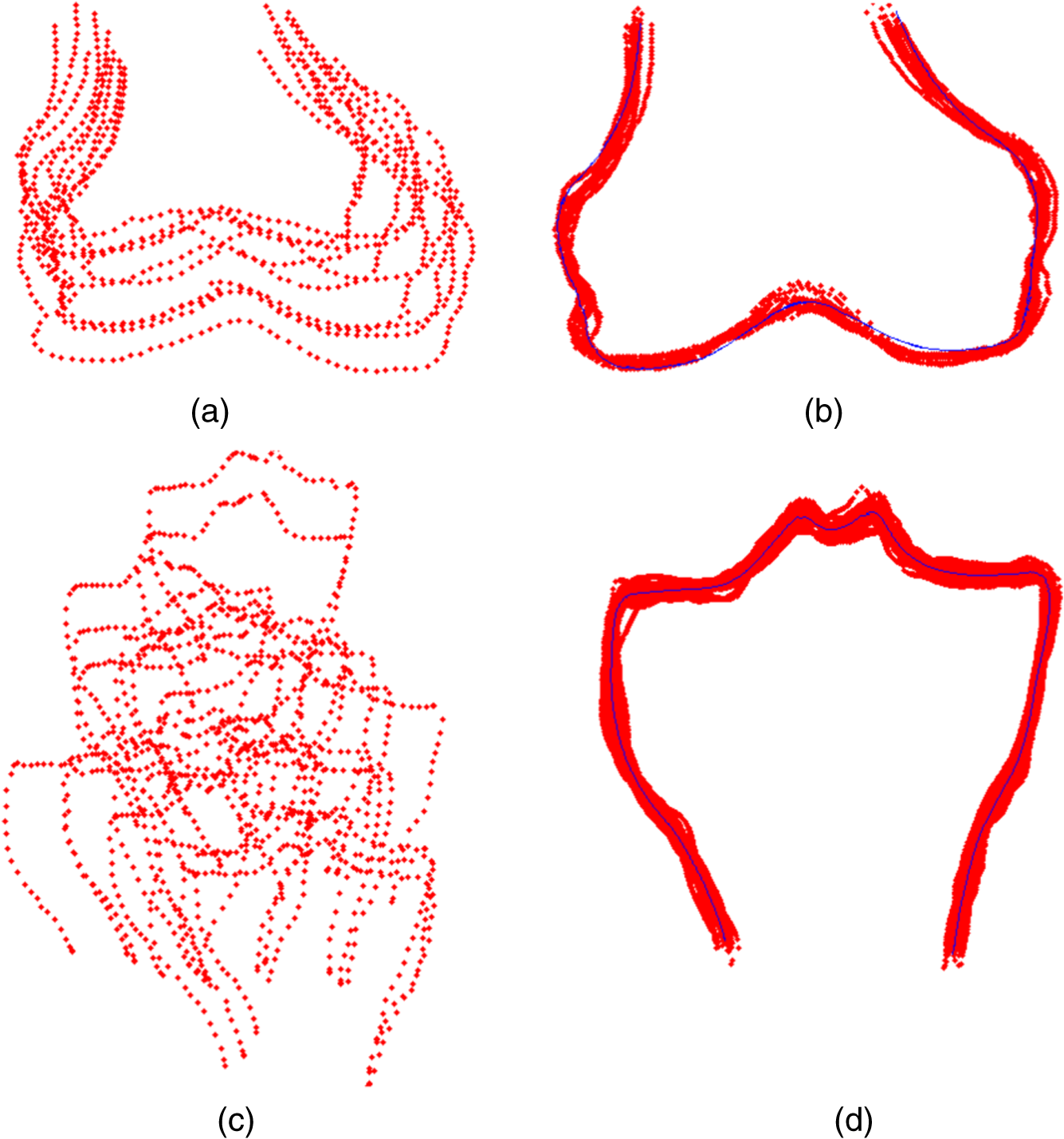

Once the training shapes have been aligned, the mean shape is calculated using $\overline{X}=\{{\overline{c}}_n|n\in \{1,\dots ,N\}\}$, where ${\overline{c}}_n=({\overline{x}}_n,{\overline{y}}_n)$ and ${\overline{x}}_n=(1/K)\sum _{\alpha }{x}_m^{\alpha }$ and ${\overline{y}}_n=(1/K)\sum _{\alpha }{y}_m^{\alpha }$, where $K$ is the number of points in each contour.

Subsequently, PCA is applied to the training dataset,¹⁰ so that any valid bone shape $\mathbf{x}$ can be represented as

Eq. (5)

$$\mathbf{x}=\overline{\mathbf{x}}+{\mathbf{\phi }}_s\mathbf{b},$$

where $\overline{\mathbf{x}}$ is the mean model, and ${\mathrm{\Phi }}_s=({\phi }_1,{\phi }_{2,}\dots ,{\phi }_m)$ is a matrix of eigenvectors corresponding to the $m$ largest eigenvalues ${\lambda }_i$ derived from the covariance matrix, $S=[1/(n-1)]\sum _{i=1}^n(x_{i-}\overline{x}){(x_{i-}\overline{x})}^T$. $m$ is chosen to be the smallest number representing more than 99% of the variance of the training set, i.e., satisfying $\sum _{i=1}^m{\lambda }_i/\sum _{i=1}^n{\lambda }_i>0.99$. $n$ is the total number of eigenvectors. These eigenvectors, ${\mathrm{\Phi }}_i$, represent the orthogonal basis of linear deformation modes that describe how points tend to move together as the shape varies. The corresponding eigenvalue ${\lambda }_i$ is equal to the variance described by each linear deformation mode. The shape model parameter, $\mathbf{b}$, is computed by $\mathbf{b}={\mathbf{\phi }}_{\mathbf{s}}^{\mathbf{T}}(\mathbf{x}-\overline{\mathbf{x}})$. When fitting the model to a set of points, the values of $\mathbf{b}$ are constrained to lie within the range $\pm 3\sqrt{{\lambda }_i}$.²¹

Figure 3 depicts the statistics of shape deformation, showing that after the first few eigenvectors, the variance becomes very small; thus, the first $m$ dominant eigenvectors are adequate to build the active shape model that accounts for the variability in the contour shapes.

Fig. 3

Statistics of shape deformation. Square root of eigenvalues sorted by size (dotted line) and components of one individual vector (solid line) indicate the shape deformation.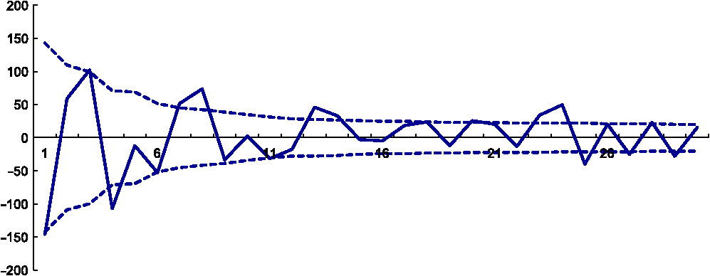

To test how ASM can model the variation of bone shape, the shape parameter was limited to fall within the range $[-3\sqrt{{\lambda }_i},3\sqrt{{\lambda }_i}]$. The eigenvector is a set of displacement vectors along, which the mean shape is deformed. To illustrate this point, the first six eigenvectors have been plotted on the mean shape in Fig. 4, resulting in the deformation from the mean shape. Due to the limitations on the number of eigenvectors and the value of shape parameters, we cannot expect ASM based on remaining examples to model the test case perfectly. The average error is $0.27\pm 0.15\mathrm{mm}$ and the maximal error is 1.10 mm. This comparison was performed by computing the RMS error of the closest corresponding points between the reconstructed contour from ASM and the original contour. The maximum error is the maximum RMS error between corresponding points of reconstructed contour from ASM and the original contour. These values represent lower limits on the errors obtained in the segmentation.

Fig. 4

(a)–(f) Mean shape deformation using first to sixth eigenvectors. The first eigenvector represents the most significant shape variation, and the contribution to shape variation decreases as the eigenvector number increases.

2.3.

Algorithm

The overall framework consists of two parts: spectral clustering for image denoising and ASM for segmentation. Spectral clustering first generates an affinity matrix from the original image.

This is followed by a solution to the generalized eigenvalue problem using a linear combination of the first $n$ eigenvectors of the affinity matrix. The output of spectral clustering is a linear combination of the eigenvectors filtered by Gaussian directional derivative filters. The segmentation part has four steps: (1) the initial contours were placed near the actual boundary by manually adjusting translation, rotation, and uniform scale. (2) An active contour search is performed to obtain the maximal gradient response in the normal profile, as shown in Fig. 5. The calculated direction of normal profile is filtered by Savitzky–Golay filter²² to get a smooth profile. (3) ASM segmentation is used to constrain the contour points in a feasible shape. (4) Relaxation is performed by the active contour search in the local neighboring area to relax the constraint from ASM so that the final boundary is on the local gradient maximum. The overall algorithm is shown in Fig. 6.

Fig. 5

The normal profile and the corresponding gradient variation: (a) gradient variation on normal profile and (b) orientation of normal profile (brown line).

Fig. 6

System framework. Spectral clustering is applied to denoise the image. ASM is applied for segmentation.

3.

Experiments and Evaluation

All images were obtained from public use datasets of the Osteoarthritis Initiative (OAI, version 0.E.1 clinical dataset; see the website at Ref. 23) of randomly selected $\sim 400$ anteroposterior knee radiographs for subjects suffering from OA. The images have been collected from different radiographic centers, resulting in large intensity differences due to the use of different x-ray and recording equipment. In addition, the presence of neighboring bones and soft tissue may result in incorrect segmentation when these artifacts have stronger edge intensities in the images than the bone of interest. Therefore, a robust automatic segmentation algorithm is important for accurate segmentation in a wide variation of x-ray images.

Experiments were designed to validate the proposed automatic segmentation algorithm. For the femur and tibia bone contours analyzed in this study, the testing images are left out and the statistical shape model is computed based on the training contours. Contours extracted from 328 x-ray images were used as the training dataset, and 80 femur and 20 tibia x-ray images were used as the testing set.

Segmentation results for each step are shown in Fig. 7. The bottom portion of the femur in Fig. 7(c) illustrates how the mistakenly segmented points in the tibia image are corrected by the ASM constraint.

Fig. 7

An example of segmentation results by spectral clustering-based ASM: (a) original image; (b) gradient search result; (c) result after ASM constraint; (d) result after relaxation; and (e) final result by convolving the contour points with a one-dimensional Gaussian filter.

Qualitative results from four examples of the validation test of the proposed automatic segmentation algorithm with respect to its capability for finding the correct femur and tibia contours are shown in Fig. 8. In these images, the ground truth (manual segmentation by an expert) is in green and the automatic segmentation is in red.

Fig. 8

Qualitative results for four cases. Green represents ground truth and red represents results from automatic segmentation algorithm.

We used dice similarity coefficient (DSC) and the root mean square (RMS) error as quantitative evaluation with respect to the capability of finding the correct object boundary. DSC is used to compare the similarity between segmented and ground truth contours.²⁴ The range of DSC is [0,1], with 0 indicating no overlapping and 1 indicating complete congruence of the two sets. DSC of the segmented femur contour is $0.97\pm 0.01$ with the worst case 0.93. DSC of the segmented tibia contour is $0.98\pm 0.01$ with the worst case 0.95. Because DSC measures the overlap ratio between the automatically and manually segmented contours, the above results indicate good overlapping of the automatic segmentation with the manual segmentation.

We compared RMS error between the original ASM algorithms, ASM with relaxation, ASM combined with MD, and the proposed algorithm (spectral clustering-based ASM). This comparison was performed by computing RMS error of the closest corresponding points between manually and automatically segmented contours. The maximum error is the maximum RMS error between corresponding points of aligned contours from automatic and manual segmentation. Totally, 80 images were used for femur testing and 20 images for tibia. Ideally, these distances are zero for a perfect fit when the automatic segmentation is the same as the manual segmentation. Table 1 shows the RMS error, its standard deviation and maximum error in millimeters.

Table 1

Comparison of performance: original ASM, ASM with relaxation, ASM with MD, and spectral clustering-based ASM.

The robustness of the proposed automatic segmentation algorithm was examined with respect to the presence of neighboring bones and low image contrast. The segmentations with and without ASM, shown in Figs. 9(b) and 9(c), demonstrate that ASM avoids infeasible points when incorrect segmentation occurs at the neighboring bone.

Fig. 9

Segmentation result with the presence of neighboring bones: (a) original image; (b) segmentation with ASM; and (c) segmentation without ASM.

4.

Conclusions

This research presents a robust automatic segmentation algorithm combining statistical shape models and spectral clustering with the objective of accurately segmenting distal femur and proximal tibia in x-ray images of varying quality. The results demonstrate a significant improvement in addressing previously unanswered problems, such as the existence of neighboring bones, image artifacts or inconsistencies, significant contrast variations, and interpatient anatomical femur/tibia shape variations.

The proposed method has significant implications for JSW assessment. Incorrect segmentation primarily occurs in the femoral condyle and tibia plateau, both of which impact the measurement of JSW significantly. The JSW measurement uses the interior contour of the tibia,²⁵ but the output of the proposed segmentation algorithm is the exterior contour of the tibia. However, the interior contour can be calculated as a postsegmentation step, using our result as an initial contour. Evaluation of JSW calculations is the subject of future work.