Identifying quantitative imaging features of posterior fossa syndrome in longitudinal MRI

Michaela Spiteri; David Windridge; Shivaram Avula M.D.; Ram Kumar M.D.; Emma Lewis

doi:10.1117/1.JMI.2.4.044502

23 October 2015 Identifying quantitative imaging features of posterior fossa syndrome in longitudinal MRI

Michaela Spiteri, David Windridge, Shivaram Avula M.D., Ram Kumar M.D., Emma Lewis

Author Affiliations +

Journal of Medical Imaging, Vol. 2, Issue 4, 044502 (October 2015). https://doi.org/10.1117/1.JMI.2.4.044502

Abstract

Up to 25% of children who undergo brain tumor resection surgery in the posterior fossa develop posterior fossa syndrome (PFS). This syndrome is characterized by mutism and disturbance in speech. Our hypothesis is that there is a correlation between PFS and the occurrence of hypertrophic olivary degeneration (HOD) in structures within the posterior fossa, known as the inferior olivary nuclei (ION). HOD is exhibited as an increase in size and intensity of the ION on an MR image. Longitudinal MRI datasets of 28 patients were acquired consisting of pre-, intra-, and postoperative scans. A semiautomated segmentation process was used to segment the ION on each MR image. A full set of imaging features describing the first- and second-order statistics and size of the ION were extracted for each image. Feature selection techniques were used to identify the most relevant features among the MRI features, demographics, and data based on neuroradiological assessment. A support vector machine was used to analyze the discriminative features selected by a generative k-nearest neighbor algorithm. The results indicate the presence of hyperintensity in the left ION as the most diagnostically relevant feature, providing a statistically significant improvement in the classification of patients (p=0.01) when using this feature alone.

1. Introduction

The posterior fossa is the most common site for intracranial tumors in children. Up to 1 in 4 children who undergo brain tumor resection surgery in the posterior fossa develop a syndrome known as posterior fossa syndrome (PFS).¹ This syndrome, also known as cerebellar mutism syndrome, describes a set of neurological symptoms that may develop from 24 to 107 h after surgery.²^,³ Children suffering from PFS characteristically suffer from disturbance in speech and mutism but may also suffer from loss of muscle tone, incontinence, strabismus (cross-eyed), dysphagia, and personality changes such as anger, apathy, melancholy, crying, and screaming.² The development of such a syndrome in children hinders their development and highly impacts their quality of life. Although PFS is a postsurgical complication, the exact underlying pathophysiological mechanism remains unclear, although it is widely considered to involve disruption of the proximal efferent cerebellar pathways (pECP) that connect the cerebellum to the forebrain. In order to reduce the incidence of PFS and manage children with this disorder, it is important to identify imaging biomarkers that are associated with it.

Our hypothesis, based on qualitative interpretation of imaging and clinical experience, is that there is a correlation between PFS and the occurrence of hypertrophic olivary degeneration (HOD) in structures known as the inferior olivary nuclei (ION). These structures, shown in Fig. 1, are paired nuclei in the brain stem, which send efferent outputs to the cerebellum, and receive inputs from the pECP. HOD is exhibited as an increase in size and intensity of the ION on an MR image that in routine clinical practice is identified qualitatively by a neuroradiologist.⁴ Qualitatively, HOD appears a number of months after surgery on routine postoperative surveillance imaging, i.e., well after the patient is diagnosed with PFS. We thus hypothesize that HOD represents the “smoking gun” that a preceding damaging event to the relevant pathways connected to the ION has occurred.

Fig. 1

Hypertrophic olivary degeneration: (a) unilateral case and (b) bilateral case.

Intraoperative MRI (IoMRI) is increasingly used to ensure the tumor is removed safely, e.g., in the resection of posterior fossa tumors. IoMRI is used during posterior fossa tumor resection. The use of IoMRI increases the likelihood that the entire tumor is removed and hence increases the likelihood of success after surgery,⁵^,⁶ but PFS can occur after attempting total resection of tumor causing injury to important structures. Furthermore, the final MR scan acquired using IoMRI provides quantitative information about the state of the ION immediately after the surgical procedure.

In the present study, we propose the quantification of HOD using longitudinal imaging features with the aim of identifying imaging features that correlate with the incidence of PFS in children. The aim was to analyze and compare imaging features in the ION on a longitudinal MRI dataset with the intention of establishing a link between PFS and HOD. Association of HOD and PFS will add to the existing evidence on the development of PFS and potentially lead to a deeper understanding of the pathogenesis of the syndrome. Segmentation was applied to the IONs on each image in the longitudinal datasets, and quantitative features were chosen to describe longitudinal changes in the area and intensity of the left and right IONs. Feature selection techniques were applied to these features in order to identify the optimal feature set. A classification model was applied to the original feature set as well as the optimized feature subsets to demonstrate the improvement in classification accuracy when using the optimized feature subsets.

2. Study Dataset

The dataset was compiled from 28 of the total patients treated for various histological types of posterior fossa tumors at Alder Hey Children’s Hospital between 2007 and 2013. The patients were aged between 8 months and 18 years old (at surgery), nine of whom were diagnosed with PFS as reported qualitatively by a consultant neuroradiologist who was blinded to the child’s neurological condition. There exist two schema for diagnosis: sensitive PFS and specific PFS. This study is based on correlating HOD to the specific diagnosis; however, it is worth noting that two additional patients within the dataset were also diagnosed with sensitive PFS. The methodology of this study did not require research ethics approval and instead was given institutional approval by the director of research at Alder Hey.

Thirteen of these patients exhibited HOD, nine bilaterally (in both ION), and four unilaterally (in either the left or right ION). Follow-up MR images during 1 year postsurgery were reviewed and up to five MR images were acquired longitudinally for each patient across their treatment. A small subset of these datasets included intraoperative MR images. Table 1 describes the MR dataset acquired for each patient, showing the number of days after surgery when an MR image was acquired. Negative numbers indicate a preoperative MR image, while intraoperative scans are indicated as ${IO}_{1}$ or ${IO}_{2}$ . Intraoperative scans were acquired to determine whether the surgical aim had been achieved. If the surgical aim was not achieved, some patients had further resections and intraoperative scans. The first intraoperative scan is indicated as ${IO}_{1}$ and the second intraoperative scan is indicated as ${IO}_{2}$ . Preoperative scans acquired on the day of the surgery are indicated as 0. Most patients were followed up every 3 months, while others with potentially malignant tumors were followed up more frequently. A mean of $4 \pm 1$ MR images was acquired for each patient with a mean time interval of $109 \pm 62$ days between each image acquisition. The age column refers to the patient’s age at surgery. Patients who were diagnosed with HOD (as determined by expert radiological assessment) are indicated as a 1, while those who did not develop HOD are indicated as a 0. Similarly, patients were categorized according to whether HOD occurred bilaterally (Bi-l) or unilaterally (Uni-l), and whether the patient was clinically diagnosed with PFS by a neurologist.

Table 1

Patient longitudinal dataset.

Pt	Image acquisition: days after surgery						Gender	Age	HOD	Bi-l	Uni-l	PFS
1	1	110	194	—	—	—	M	4	0	0	0	0
2	121	205	289	401	—	—	F	7	1	1	0	0
3	120	204	288	400	—	—	M	6	0	0	0	0
4	1	77	118	—	—	—	F	0	0	0	0	0
5	1	98	231	413	—	—	F	4	0	0	0	0
6	$- 30$	0	175	287	403	—	F	4	0	0	0	0
7	143	318	437	—	—	—	M	3	1	1	0	0
8	118	278	481	—	—	—	M	7	1	0	1	0
9	176	260	372	—	—	—	F	7	1	1	0	1
10	189	273	357	—	—	—	F	7	1	0	1	0
11	$- 1$	2	96	193	216	334	M	3	0	0	0	0
12	91	228	351	—	—	—	F	8	1	1	0	1
13	18	21	165	228	—	—	F	14	1	0	1	0
14	${IO}_{1}$	76	87	28	60	—	F	2	0	0	0	0
15	136	257	440	—	—	—	F	5	1	1	0	0
16	89	285	—	—	—	—	M	1	0	0	0	0
17	313	481	—	—	—	—	F	6	1	1	0	1
18	${IO}_{1}$	110	446	—	—	—	F	10	0	0	0	0
19	124	288	481	—	—	—	M	17	1	1	0	1
20	97	181	321	—	—	—	F	12	1	1	0	1
21	${IO}_{1}$	${IO}_{2}$	108	255	445	—	M	11	0	0	0	0
22	${IO}_{1}$	${IO}_{2}$	125	—	—	—	M	3	0	0	0	0
23	131	299	—	—	—	—	F	15	1	1	0	1
24	${IO}_{1}$	19	201	322	—	—	F	14	0	0	0	0
25	$- 2$	${IO}_{1}$	${IO}_{2}$	173	509	—	M	13	0	0	0	0
26	184	228	—	—	—	—	F	3	1	0	1	1
27	${IO}_{1}$	${IO}_{2}$	178	273	424	—	M	8	0	0	0	1
28	${IO}_{1}$	1	110	292	—	—	F	7	0	0	0	1
Key
HOD			Presence of HOD							$1 = yes$ , $0 = no$
Bi-l			Presence of bilateral HOD							$1 = yes$ , $0 = no$
Uni-l			Presence of unilateral HOD							$1 = yes$ , $0 = no$
PFS			PFS diagnosis							$1 = yes$ , $0 = no$

T2-weighted sequences from the pre-, intra-, and postoperative scan were used to evaluate for HOD, and the following parameters were used: $TR = 4485 ms$ , $TE = 11 ms$ , $slice thickness = 6 mm$ , $number of slices = 20$ , $time step = 4.49 s$ . The preoperative and postoperative MR images were acquired using 1.5 T or 3 T magnets. Intraoperative MR images were acquired using 3 T magnets. This modality was used due to its ability to identify cerebrospinal fluid, blood, and edema as increased gray-level intensity. The T1 MR images obtained for these patients were not analyzed as they do not provide sufficient information relating to hypertrophy in the ION.

T2 volumetric imaging is not routinely used as it is time-consuming and prone to movement-associated artifacts. Instead, axial T2 spin-echo sequences were used to evaluate for HOD as they result in the best signal and contrast resolution to assess the ION. These T2 MR images were acquired in spiral MRI, which captures the k-space through a spiral trajectory. This method of acquisition is fast and results in high in-plane spatial resolution, giving improved resolution of small structures within the brain, specifically the ION.⁷^,⁸

3. Methodology

The aim of this study is to identify biomarkers that correlate with the development of PFS following tumor resection surgery in the posterior fossa. In order that these biomarkers may aid understanding of the pathogenesis of PFS, techniques have been chosen to ensure that comprehensibility of imaging and clinical features is retained throughout the pipeline. This study consists of four stages: image preprocessing, feature extraction, feature selection, and classification. The features were chosen to quantify HOD, namely, an increase in intensity and size, in the left or right ION.

3.1.

Image Preprocessing

In order to extract information (features) about each ION, it was necessary to segment these structures on the MR images. Images were acquired with spiral MRI; therefore, a full volumetric representation was not obtained. For this reason, segmentation was performed on two-dimensional image slices.

The non-HOD ION cannot be clearly delineated by the naked eye on MRI. This is due to very low contrast with the surrounding tissue as well as its relatively small cross-sectional area. For this reason, segmentation was carried out using a semiautomated seed-growing technique in two-dimensional space. The right and left ION were segmented separately. Images were registered to Talaraich space, using a rigid body affine transformation, with intensity scaling, prior to segmentation.

The process by which segmentation is carried out consists of three main steps: (1) an arbitrary seed-point within the ION was manually identified using prior anatomical knowledge—the IONs are on the anterior part of the brain stem, located on either side of its midline (when the IONs are hypertrophic their gray-level intensity is relatively higher than surrounding brain stem tissue and are therefore easier to identify); (2) region growing from a seed-point, with intensity $I_{s}$ , was performed by analyzing pixels in a search space of a 4 mm radius: a pixel within the search space is included in the region of interest (ROI) if its gray-level intensity, $I_{p}$ , lies within the range $| I_{p} \pm T | \leq | I_{s} |$ , and its difference from adjacent pixels, $I_{a}$ , lies within the range $| I_{a} | \leq | I_{p} \pm T |$ , where $T$ is a threshold that was varied between 12 and 16 heuristically until the ROI did not vary in shape or size;⁹ (3) the application of a morphological closing-operation using a full-width at half-maximum of 4 mm and a threshold of 0.5.⁹

These steps are applied iteratively until no further change occurs in the ROI. The segmentation process was carried out three times for each MR image in order to assess intraobserver variability. The first segmentation dataset was validated and amended by an expert neuroradiologist. This introduced a measure of interobserver variability as the first segmentation test set was expertly validated, while the other two segmentation test sets were not.

3.2.

Feature Extraction

Once the desired region was segmented, it was possible to extract a set of features from each ION. HOD is characterized by an increase in volume of the ION, which can be seen as both an enlargement and an increase in signal intensity on a T2-weighted MR image. Imaging features related to an increase in size and image intensity are extracted from the MR images. The area of the left and right IONs is obtained as well as the contrast between the left and right IONs and surrounding brain stem tissue within the same MR image slice.

The contrast was calculated using the definition of Weber contrast ( $W$ )

Eq. (1)

W = \frac{I_{ION} - I_{b}}{I_{b}},

where

I_{ION}

refers to the mean gray-level intensity of the ION and

I_{b}

refers to the mean gray-level intensity of the surrounding tissue

For each MRI, the contrast of both the left and right IONs was calculated separately. The segmentation of the left and right IONs is exhibited in Fig. 2.

Fig. 2

Segmentation of inferior olivary nuclei (delineated in black): (a) unilateral case and (b) bilateral case.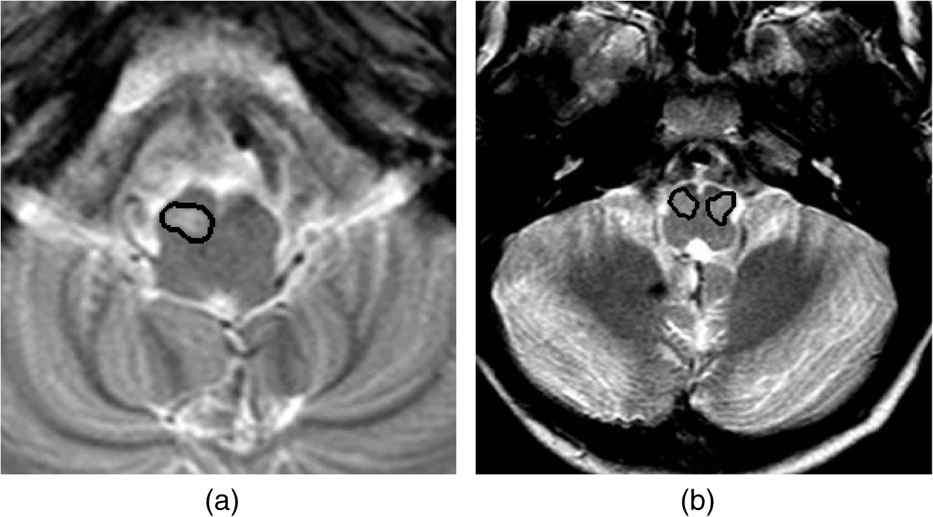

The imaging features are chosen to relate to physiological characteristics of HOD, namely, a change in intensity with respect to surrounding brain stem tissue and an increase in area of the left and right IONs, respectively. It was desired to quantify these characteristics longitudinally.

The contrast, defined in Eq. (1), for both the left and right IONs, $C_{L}$ and $C_{R}$ , was obtained for up to 6 MR images per patient acquired at different time points throughout each patient’s treatment. The mean gradient of contrast against time was calculated, symbolized by $mean (Δ C_{L} / Δ t)$ and $mean (Δ C_{R} / Δ t)$ , respectively. The variance of gradient of contrast against time, $var (Δ C_{L} / Δ t)$ and $var (Δ C_{R} / Δ t)$ , was also calculated across each patient’s longitudinal set of MR images.

Similarly, the area of the ION was calculated from each MRI and the mean slope and variance across each longitudinal dataset for the left and right IONs separately. These values are symbolized by $mean (Δ A_{L} / Δ t)$ , $mean (Δ A_{R} / Δ t)$ , $var (Δ A_{L} / Δ t)$ , and $var (Δ A_{R} / Δ t)$ .

Features determined by expert radiological assessment of each MR image were also included, namely, whether HOD is present (1) or not (0), whether HOD is present unilaterally (1) or not (0), and whether HOD is present bilaterally (1) or not (0). The neuroradiologist was blinded to the PFS status of the patient. It is important to note that these features are not mutually exclusive, and the lack of presence of HOD bilaterally may imply either unilateral HOD or no HOD.

The features included are shown in Table 2. Features (1) to (8) are obtained from MR data, features (9) to (14) represent clinical data. Features (15) and (16) represent random noise added in order to assess the discriminative ability of the feature selection algorithms used later.

Table 2

Features included.

Feature	Definition
1	$mean (Δ C_{L} / Δ t)$
2	$var (Δ C_{L} / Δ t)$
3	$mean (Δ A_{L} / Δ t)$
4	$var (Δ A_{L} / Δ t)$
5	$mean (Δ C_{R} / Δ t)$
6	$var (Δ C_{R} / Δ t)$
7	$mean (Δ A_{R} / Δ t)$
8	$var (Δ A_{R} / Δ t)$
9	Presence of HOD
10	Bilateral HOD
11	Unilateral HOD
12	Enlargement
13	Gender
14	Age at surgery
15	Random noise 1
16	Random noise 2

3.3.

Feature Selection

Dimensionality reduction techniques, such as principal component analysis (PCA), result in loss of comprehensibility from the point of view of a clinical practitioner,¹⁰ rendering it inappropriate for this application due to the need for medics and clinicians to interpret results. PCA identifies linear combinations of features as opposed to discrete ones and is therefore less applicable to diagnosis.

From a machine-learning respective, to avoid the classifier over fitting the data, in the case of too many features, it is desirable to use only the most relevant features in classifying data into two groups: patients who have developed PFS and those who have not. We, however, have an additional motivation; the determination of diagnostically relevant medical indicators. This is known as feature selection and can be carried out using filter or wrapper methods.¹¹^,¹²

In general, the problem of feature selection is NP-hard and therefore intractable for large datasets. Various techniques have therefore been applied; however, these are all prone to local minima. The most common techniques used to identify the salient features out of the full feature set are random subset feature selection (RSFS), sequential forward selection (SFS), and sequential floating forward selection (SFFS).¹³^,¹⁴

For each feature selection algorithm, a subset of features is chosen and classification is carried out as a criterion for selecting the optimal features. A k-nearest neighbor (k-NN) classifier was used in each algorithm as it is a generative technique that follows the underlying distribution of data. A support vector machine (SVM, used for classification in Sec. 3.4) was not ideal for this task, as it is a discriminative technique and hence more ideal for binary diagnostic classification. The relevance of each feature was scored using a UAR as in the case of the RSFS algorithm.¹³^,¹⁴

RSFS chooses a random subset of features from the entire feature set, the size of which is equal to the square root of the total number of features. A k-NN classification using three neighbors is carried out repeatedly on this chosen subset. Each feature is given a relevance score that is continuously updated according to its inclusion in the random subsets that perform well.¹³^,¹⁵ The relevance values of each feature are compared to random walk statistics, and good features are chosen accordingly. The algorithm is carried out until the stopping criterion is reached, i.e., if the size of the final feature set (consisting of the features with the highest relevance scores) has not changed by more than 0.5% in the previous 1000 iterations, or if the maximum number of iterations (300,000) is reached. The RSFS algorithm was carried out 100 times, each time randomly dividing the dataset in two.

Unlike RSFS, SFS starts off with an empty dataset. One feature is added at a time and a feature is kept or discarded depending on whether it exhibits the best classification performance when used together with the previously chosen features. SFS also makes use of k-NN classifier on the feature subset in order to obtain a classification score. Low-scoring features were discarded. In SFFS, an attempt is made at finding the least useful feature in order to discard it from the final feature set. This process is repeated until the evaluation score becomes (and remains) better than the previous best score using a feature set of the same size.¹³^,¹⁴ Both the SFS and SFFS algorithms were carried out using three neighbors, four neighbors, five neighbors, and six neighbors. This process was carried out 100 times, and the average relevance scores were calculated.

All three-feature selection methods were carried out on three separate segmentation test sets in order to assess differences in scores that may arise due to intraobserver and interobserver variability.

3.4.

Classification

The binary classification was carried out in order to assess the discriminative ability of the most relevant features chosen in the previous stage of the study. The aim is to classify patients into two groups: patients who developed PFS and patients who had not developed PFS.

Two different feature subsets were used: the first subset included the entire feature set, while the second subset included the most relevant features chosen by the RSFS, the SFS, and SFFS algorithms. A simple linear nonkernelized SVM was used to perform the classification task. SVM is a state-of-the-art classification model used for binary classification when the dataset falls into two main categories (SVMs).¹⁶^,¹⁷

Due to the small size of the dataset, it was not feasible to split the data into training data and test data. Since there is no natural division between training and test sets within the data, the most efficient and ideal way to maximize the use of this small dataset was to implement a leave-M-out cross-validation. In this validation technique, M observations are omitted from the entire set for training purposes; the M observations are then used as the test set; this process is repeated a number of times in order to obtain a mean value for the area under the curve (AUC) and the accuracy of the SVM classifier. A leave-eight-out cross-validation for each feature subset was carried out 100,000 times. For each permutation, the SVM bias was varied between $- 4$ and 4, in increments of 0.2. The false positives and the false negatives were obtained for each bias point, and a mean of these values across all the permutations was obtained. Receiver operating characteristic (ROC) graphs, exhibiting the false positives against the true positives, were plotted in order to assess the difference in classification accuracy when using different feature subsets; the area under the ROC curves was obtained. A leave-one-out cross-validation was carried out for all the patients (28 times) in order to obtain a mean accuracy score for each feature subset.

4. Results

4.1.

Features

Table 3 exhibits the mean, $μ$ , and standard deviation, $σ$ , for features 1 to 8, for segmentation test sets 1, 2, and 3.

Table 3

The mean and standard deviation of the imaging features for segmentation test sets 1, 2, and 3.

μ±σ(×10−4)
Feature	1	2	3	4	5	6	7	8
Test	mean(ΔCL/Δt)	var(ΔCL/Δt)	mean(ΔAL/Δt)	var(ΔAL/Δt)	mean(ΔCR/Δt)	var(ΔCR/Δt)	mean(ΔAR/Δt)	var(ΔAR/Δt)
1	$- 2.26 \pm 4.17$	$75.48 \pm 82.89$	$0.51 \pm 1.41$	$10.17 \pm 19.58$	$- 1.20 \pm 5.64$	$105.49 \pm 96.98$	$0.63 \pm 1.49$	$12.40 \pm 25.55$
2	$- 1.64 \pm 3.19$	$80.13 \pm 91.00$	$- 0.23 \pm 0.78$	$3.59 \pm 3.36$	$1.16 \pm 6.35$	$89.29 \pm 107.60$	$0.04 \pm 0.93$	$3.79 \pm 2.85$
3	$- 1.21 \pm 4.45$	$66.30 \pm 56.75$	$0.85 \pm 1.18$	$7.43 \pm 11.64$	$- 0.20 \pm 5.08$	$86.10 \pm 66.81$	$0.34 \pm 1.14$	$6.85 \pm 12.13$

4.2.

Feature Selection

Table 4 shows the relevance scores calculated by the RSFS algorithm. Table 5 displays the relevance scores calculated by the SFS algorithm, and Table 6 displays the relevance scores calculated by the SFFS algorithm using a k-NN classifier with 3, 4, 5, and 6 neighbors; these algorithms yielded identical results. Feature 1 consistently obtained the highest score for all feature selection techniques.

Table 4

The relevance scores calculated by the random subset feature selection algorithm.

Average relevance score over 100 iterations
	Feature key
Test	1	2	3	4	5	6	7	8	9	10	11	12	13	14	15	16
1	6.22	1.61	1.08	1.81	1.64	0.23	0.65	0.11	1.06	0.94	0.16	0.03	0.42	0.09	0.00	0.00
2	8.99	0.09	0.31	1.41	1.03	0.20	0.28	1.22	0.92	1.77	0.27	0.10	1.28	0.30	0.00	0.00
3	10.03	1.24	0.00	0.42	0.00	0.12	1.62	0.15	1.19	1.46	0.00	0.00	0.18	0.59	0.00	0.00

Table 5

The average relevance scores calculated by the sequential forward selection algorithm over 100 iterations.

Average relevance score over 100 iterations
Test	Feature key	k=3	k=4	k=5	k=6
1	1	68.38	72.68	74.10	71.37
2	1	77.93	76.04	73.37	69.77
3	1	85.10	85.31	85.87	86.34

Table 6

The average relevance scores calculated by the sequential floating forward selection algorithm over 100 iterations.

Average relevance score over 100 iterations
Test	Feature key	k=3	k=4	k=5	k=6
1	1	68.88	75.32	73.88	73.22
2	1	76.75	77.56	74.34	71.48
3	1	84.98	85.18	85.87	86.39

4.3.

Classification

Figure 3 exhibits the ROC curve for the SVM classifier used in the full feature dataset and feature 1, the most relevant feature found using the RSFS, SFS, and SFFS algorithms.

Fig. 3

The receiver operating characteristic (ROC) curve for the support vector machine classifier used on the full feature dataset and feature 1 on test sets 1, 2, and 3.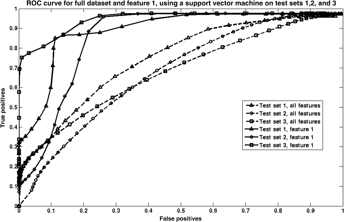

Table 7 reports the AUC for the SVM classifier for all three segmentation test sets carried out on the full feature set and feature 1, as well as the average AUC and accuracy for the full feature set and feature 1. A paired $t$ -test was carried out to calculate the significance of the difference between the AUCs of the three ROC curves when considering feature 1, and the three ROC curves when considering the whole feature set for test sets 1, 2, and 3. The confidence interval was taken to be 95%. The two-tailed $p$ -value was found to be 0.01.

Table 7

Area under the curve (AUC) and accuracy for the support vector machine classifier used on the full feature dataset and feature 1 on test sets 1, 2, and 3.

	AUC		Accuracy (%)
Test	Full feature set	Feature 1	Full feature set	Feature 1
1	0.74	0.89	78.57	89.29
2	0.62	0.85	75.00	78.57
3	0.64	0.89	71.43	85.71
Average	0.67	0.88	75.00	84.52

5. Discussion

The results yielded by the RSFS algorithm in Table 4 indicate feature 1 as the most relevant feature, scoring higher than all other features considered in this study. This feature corresponds to the mean slope of contrast in the left nucleus. The score for this feature in each test set was 6.22, 8.99, and 10.03 for test sets 1, 2, and 3, respectively. These scores are at least five times higher than the scores for all the other features in the full feature set.

These results indicate that changes in contrast in the left ION are the most relevant feature correlating with the development of PFS. This implies that change in intensity of the left ION as seen on MRI is highly correlated to the presence of PFS. This quantified contrast in the left ION from patient MR is at least six times as predictive as the diagnosis of HOD made by radiological assessment as a predictor of PFS. Feature 1 is linked to HOD, as a high value for $mean (Δ C_{L} / Δ t)$ , indicates increasing hyperintensity over time in the left ION and therefore the presence of HOD in the left ION. This finding suggests that an overall increase in contrast over time between the left ION tissue and surrounding brain stem tissue indicates the development of PFS, irrespective of whether the HOD is unilateral or bilateral, and whether the left or the right ION is brighter at any point throughout the patient’s treatment. These findings are in keeping with the results of a recent study where damage to the right efferent cerebellar pathway, which communicates with the left ION, had a significant association with the development of PFS.⁴^,¹⁸^,¹⁹

The results yielded by SFS and SFFS, exhibited in Tables 5 and 6, also indicate feature 1 as the most relevant feature, with all other features scoring negligible relevance scores in comparison to feature 1. Feature 1 consistently scored 68.38 or higher throughout all four tests ( $k = 3$ , 4, 5, and 6) for all the segmentation test sets. The relevance scores for the other features in the feature set scored at least 70 times lower. This further proves the relevance of an increase in intensity of the left ION in the onset of PFS.

It should be noted that the search strategies used in this study are not optimal and are prone to local minima, with the exception of SFFS which makes an attempt at eliminating irrelevant features by carrying out a backward search in addition to the forward search. Notwithstanding this, the feature selection methods carried out in this study are ideal in a clinical scenario, more than other methods, such as PCA, as the features retain interpretability after the feature selection techniques are applied.

The results yielded by the SVM classifier, shown in Fig. 3, show an increase in classifier accuracy as the least diagnostically relevant features were eliminated. The SVM classifier reached an accuracy of 89.29%, 78.57%, and 85.71%, respectively, for each segmentation test set, when the only feature included was the one selected by the RSFS, SFS, and SFFS algorithms, i.e., quantified contrast in the left ION. The AUC was also optimized when classification was carried out using feature 1, with values of 0.89, 0.85, and 0.89 for segmentation test sets 1, 2, and 3, respectively.

From Table 7, it is evident that for each segmentation test set, the AUC and the accuracy are increased when only feature 1 is used. The $p$ -value measuring the difference between the AUCs for the full feature set and the AUCs for feature 1 is statistically significant by conventional criteria. This implies that the performance of the SVM classifier is improved if only feature 1 is considered.

The average slope of contrast in the left ION is obtained by image analysis and is therefore objective, while the diagnosis of HOD (by radiological assessment) is made by human assessment and is subjective and prone to human error. This shows that quantified contrast in the left ION can be used a biomarker for PFS following posterior fossa tumor resection. This is one of the pioneering studies correlating HOD and PFS using semiautomated image analysis. A previous study exists; however, it did not make use of semiautomated image analysis and instead relied on human observation to identify HOD in each MRI. Such analysis is subjective and prone to human error.⁴

6. Conclusion

The aim of the experiment was to investigate the link between PFS and HOD in order to build upon the existing evidence on the development of PFS and to lead to a deeper understanding of the pathogenesis of the syndrome. A dataset of 28 patients was included in this study. The main contribution of this work consists of the quantification of HOD using automated imaging feature extraction to describe changes in intensity and size of the ION longitudinally.

This study has identified intensity, or $mean (Δ C_{L} / Δ t)$ , in the left ION as the most diagnostically relevant feature that correlates with the development of PFS following tumor resection in the posterior fossa.

Other features, including clinical features, consistently scored lower than the average slope of contrast in the left ION, throughout this study. Our findings indicate that the presence of HOD, specifically in the left ION, is highly associated with the onset of PFS following tumor resection surgery in the posterior fossa. These findings lend quantitative support to our hypothesis that there is a correlation between PFS and the occurrence of HOD following tumor resection in the posterior fossa, based on qualitative assessment of imaging. These results suggest common anatomical substrates involved in the development of PFS and HOD and indicate an element of laterality in the development of this syndrome. This is the first study to quantify HOD using semiautomated image analysis adding reproducible and quantitative evidence to the proven hypothesis that HOD correlates with PFS.

Acknowledgments

We acknowledge the support of the Rabin Ezra Scholarship Fund in the form of a bursary, which enabled the open-access publication of this paper.

References

1.

J. Siffert et al., “Neurological dysfunction associated with postoperative cerebellar mutism,” J. Neurooncol., 48 75 –81 (2000). http://dx.doi.org/10.1023/A:1006483531811 Google Scholar

2.

E. A. Kirk, V. C. Howard and C. A. Scott, “Description of posterior fossa syndrome in children after posterior fossa brain tumor surgery,” J. Pediatr. Oncol. Nurs., 12 (4), 181 –187 (1995). http://dx.doi.org/10.1177/104345429501200402 JONUEM Google Scholar

3.

H. Baillieux et al., “Posterior fossa syndrome after a vermian stroke: a new case and review of the literature,” Pediatr. Neurosurg., 43 386 –395 (2007). http://dx.doi.org/10.1159/000106388 PDNEEV Google Scholar

4.

Z. Patay et al., “MR imaging evaluation of inferior olivary nuclei: comparison of postoperative subjects with and without posterior fossa syndrome,” Am. J. Neuroradiol., 35 (4), 797 –802 (2013). http://dx.doi.org/10.3174/ajnr.A3762 Google Scholar

5.

M. R. Chicoine et al., “Implementation and preliminary clinical experience with the use of ceiling mounted mobile high field intraoperative magnetic resonance imaging between two operating rooms,” Acta Neurochir. Suppl., 109 97 –102 (2011). http://dx.doi.org/10.1007/978-3-211-99651-5_15 Google Scholar

6.

N. Sannai and M. S. Berger, “Operative techniques for gliomas and the value of extent of resection,” Neurotherapeutics, 6 478 –486 (2009). http://dx.doi.org/10.1016/j.nurt.2009.04.005 Google Scholar

7.

H. Tan, “Estimation of k-space trajectories in spiral MRI,” Magn. Reson. Med., 61 1396 (2009). http://dx.doi.org/10.1002/mrm.21813 MRMEEN 0740-3194 Google Scholar

8.

B. M. A. Delattre et al., “Spiral demystified,” Magn. Reson. Imaging, 28 (6), 862 –881 (2010). http://dx.doi.org/10.1016/j.mri.2010.03.036 MRIMDQ 0730-725X Google Scholar

9.

C. Rorden and M. Brett, “Stereotaxic display of brain lesions,” Behav. Neurol., 12 191 –200 (2000). http://dx.doi.org/10.1155/2000/421719 BNEUEI Google Scholar

10.

S. Karamizadeh et al., “An overview of principal component analysis,” J. Signal Inf. Process., 4 173 –175 (2013). http://dx.doi.org/10.4236/jsip.2013.43B031 Google Scholar

11.

G. H. John, R. Kohavi and K. Pfleger, “Irrelevant features and the subset selection problem,” in Proc. of the Int. Conf. on Machine Learning, 121 –129 (1994). Google Scholar

12.

I. Kojadinovic and T. Wottka, “Comparison between a filter and a wrapper approach to variable subset selection in regression problems,” (2000). Google Scholar

13.

J. Pohjalainen, O. Räsänen and S. Kadioglu, “Feature selection methods and their combinations in high-dimensional classification of speaker likability, intelligibility and personality traits,” Comput. Speech Lang., 29 (1), 145 –171 (2014). http://dx.doi.org/10.1016/j.csl.2013.11.004 CSPLEO 0885-2308 Google Scholar

14.

A. W. Whitney, “A direct method of nonparametric measurement selection,” IEEE Trans. Comput., C-20 1100 –1103 (1971). http://dx.doi.org/10.1109/T-C.1971.223410 ITCOB4 0018-9340 Google Scholar

15.

O. Rasanen and J. Pohjalainen, “Random subset feature selection in automatic recognition of developmental disorders, affective states, and level of conflict from speech,” in Proc. Interspeech ’2013, (2013). Google Scholar

16.

C. Campbell, “Kernel methods: a survey of current techniques,” Neurocomputing, 48 (1–4), 63 –84 (2002). http://dx.doi.org/10.1016/S0925-2312(01)00643-9 NRCGEO 0925-2312 Google Scholar

17.

J. Shawe-Taylor and N. Cristianini, Kernel Methods for Pattern Analysis, Cambridge University Press, Cambridge (2004). Google Scholar

18.

N. Law et al., “Clinical and neuroanatomical predictors of cerebellar mutism syndrome,” Neuro-Oncology, 14 1294 –1303 (2012). http://dx.doi.org/10.1093/neuonc/nos160 Google Scholar

19.

S. Kpeli et al., “Posterior fossa syndrome after posterior fossa surgery in children with brain tumors,” Pediatr. Blood Cancer, 56 (2), 206 –210 (2011). http://dx.doi.org/10.1002/pbc.22730 Google Scholar

Biography

Michaela Spiteri is a doctoral student in electronic engineering at the Centre for Vision, Speech, and Signal Processing, University of Surrey, UK, under Dr. Emma Lewis. Her thesis is entitled “Longitudinal MRI assessment of brain tumors in children.” Before coming to Surrey, she completed her MSc in biomedical engineering (2012 to 2013). Before that she received a BEng (HONS) in electrical and electronic engineering from University of Malta in 2012. She is a member of SPIE.

David Windridge is a senior lecturer in computer science at the Middlesex University and heads the university’s data science activities. He is a visiting professor at the Trento University, Italy, and a visiting senior research fellow at the University of Surrey (he was previously a senior research fellow within the Centre for Vision, Speech, and Signal Processing). His research interests include center on the fields of machine learning (particularly kernel methods classifier-fusion), cognitive systems, and computer vision. He has authored more than 80 peer-reviewed publications.

Shivaram Avula is a consultant pediatric radiologist at the Alder Hey Children’s Hospital with an interest in neuroimaging. He completed pediatric radiology fellowships at the Alder Hey and the Hospital for Sick Children in Toronto, Canada. His clinical interests include head and neck imaging, neuroimaging for brain tumors, epilepsy, and other childhood neurological disorders. His research interests include advanced neuro-MRI techniques for brain tumors and intraoperative MRI.

Ram Kumar has been a consultant pediatric neurologist at the Alder Hey Children’s Hospital in Liverpool since early 2007. He is the service group lead for neurology, neurosurgery, long-term ventilation, rehabilitation, and sleep services. He obtained an MA degree in pathology from University of Cambridge in 1992, a bachelor of medicine and surgery from the same university in 1994, and an MRCP (UK) in 1998. He joined the GMC specialist register CCT in pediatrics and pediatric neurology in 2007.

Emma Lewis is a lecturer in medical image analysis at the Centre for Vision Speech and Signal Processing, University of Surrey. Previously, she was a principal research fellow at the Dementia Research Centre, National Hospital for Neurology and Neurosurgery, London. Her research involves applying image-processing techniques within a variety of clinical application areas and image modalities. In particular, she has developed methods for quantification, simulation, and artifact correction within domains including neuroimaging, mammography, and nuclear medicine motion correction.

CC BY: © The Authors. Published by SPIE under a Creative Commons Attribution 4.0 Unported License. Distribution or reproduction of this work in whole or in part requires full attribution of the original publication, including its DOI.

Citation Download Citation

Michaela Spiteri, David Windridge, Shivaram Avula M.D., Ram Kumar M.D., and Emma Lewis "Identifying quantitative imaging features of posterior fossa syndrome in longitudinal MRI," Journal of Medical Imaging 2(4), 044502 (23 October 2015). https://doi.org/10.1117/1.JMI.2.4.044502

Published: 23 October 2015

Access the abstract

JOURNAL ARTICLE
9 PAGES

DOWNLOAD PAPER SAVE TO MY LIBRARY

GET CITATION

CITATIONS

Cited by 11 scholarly publications.

Explore citations on Lens.org

KEYWORDS

Ions

Magnetic resonance imaging

Image segmentation

Information operations

Tumors

Feature selection

Surgery

1.

Introduction

Fig. 1

2.

Study Dataset

Table 1

3.

Methodology

3.1.

Image Preprocessing

3.2.

Feature Extraction

Eq. (1)

Fig. 2

Table 2

3.3.

Feature Selection

3.4.

Classification

4.

Results

4.1.

Features

Table 3

4.2.

Feature Selection

Table 4

Table 5

Table 6

4.3.

Classification

Fig. 3

Table 7

5.

Discussion

6.

Conclusion

Acknowledgments

References

Biography

Show All Keywords

Keywords/Phrases

Search In:

Publication Years