1.

Introduction

In vivo diagnosis of breast cancers is often difficult because the x-ray linear attenuation coefficients $\mu$ of fibroglandular and cancerous tissue are similar.¹ Even with the advancements in medical imaging, such as digital mammography,² and three-dimensional (3-D) imaging techniques, such as breast tomosynthesis³ and cone-beam computed tomography (CBCT),⁴ suspicious lesions will continue to exist since all these imaging methods are based on detecting differences in $\mu$.

The diagnosis of suspicious lesions is routinely done via removal of tissue and its subsequent analysis via histology. The tissue samples extracted undergo a gross examination by a pathologist. Sampling errors can occur at the grossing stage and meticulous anatomic examination is required to avoid sampling the wrong part of the tissue.⁵ The number of sections cut and sampled affects the quality of the gross examination.⁵ Khaddage et al.⁶ found that it is important to analyze a greater proportion of the sectioned tissue.

Conventional tissue processing which requires fixing, dehydrating, cleaning, and impregnating the tissue with chemical reagents is time consuming (e.g., 8 h) and delays diagnosis.⁷ A rapid diagnosis could allow for earlier treatments and a better quality of life. Pathologists grade lesions based on histological classifications (e.g., benign, atypical hyperplasia, in situ carcinoma, invasive carcinoma) and evaluations should be accurate and reproducible. However, Palli et al.⁸ showed interobserver inconsistencies in assessing atypical hyperplasia (e.g., a borderline lesion with associated high risk for future cancers) and in situ carcinoma. Verkooijen et al.⁹ found discrepancies in histologic diagnoses of normal and borderline lesions between routine pathologists and an expert review panel of pathologists. Out of 718 breast specimens, the routine pathologists identified 24% (large-core needle biopsies) and 43% (open biopsies) of borderline lesions identified by the review panel. The analysis of microscopic details of tissue slides is subject to interpretation,¹⁰ which leads to intraobserver variabilities.¹¹ For example, lobular cancers in the breast form small clusters or appear as single tumor cells, and therefore are difficult to detect using conventional histological methods.¹²

Researchers are looking to devise complementary methods for diagnosing cancers in breast biopsies.^13–41

Phase constrast x-ray scatter imaging¹³ produces images based on how x-rays are refracted. A theoretical work by Feye-Treimer and Treimer¹³ showed that angular resolved phase-based scattering of x-rays might provide a technique to distinguish malignant cells from healthy ones if the cell–cell nucleus system is considered as a coherent phase shifting object.

Raman spectroscopy measures the inelastic scattering of light from tissue.^14,15 The recorded energy shifts reveal chemical information.¹⁵ Haka et al.¹⁵ examined 130 Raman spectra of breast tissue samples ($1{\mathrm{mm}}^3$) from 58 patients. Using a diagnostic algorithm, they classified normal, benign, and malignant tissue with 94% sensitivity and 96% specificity.

X-ray Compton scatter methods have been explored to assess electron densities.^16,17 Antoniassi et al.¹⁶ used $K^{\alpha }$ (17.44 keV) radiation from molybdenum and a 90-deg scatter angle to show that electron densities of adipose breast tissue were less than fibrous and neoplastic tissue. Ryan et al.¹⁷ using $K^{\alpha }$ (57.97 keV) photons from tungsten measured photons scattered at 30 deg. Differences could be seen between adipose and malignant tissue (9.0%) while the differences between malignant and fibrocystic change tissue were considered not significant (3.4%).

Primary x-ray beams incident on breast biopsies cause trace elements to emit secondary x-rays with unique wavelengths.¹⁸ Geraki et al.¹⁹ used a synchrotron x-ray fluorescence study and found statistical increases in concentrations of iron, copper, zinc, and potassium in malignant breast tissue. Pereira et al.²⁰ also observed increases in zinc and iron.

Several groups^21–41 are devising x-ray diffraction methods to detect cancers in breast biopsies. There are two regimes of interest: small-angle x-ray scatter (SAXS) ($x<0.1{\mathrm{nm}}^{-1}$)^21–28 for studying supramolecular structures and wide-angle x-ray scatter (WAXS) ($0.5{\mathrm{nm}}^{-1}<x<5{\mathrm{nm}}^{-1}$)^29–41 conventionally used to study crystallographic structures. The momentum transfer variable $x=\sin (\theta /2)/\lambda$ combines the dependence of scatter on x-ray wavelength ($\lambda$) and scatter angle ($\theta$).

In the SAXS regime, structures on the order of 10 to 100 nm are probed (e.g., within collagen, the $d$-spacing is 65 nm).^24,27 Measurements of SAXS generally require a highly focused monochromatic synchrotron beam and long sample to flat panel detector distances (e.g., 10 m). Sidhu et al.²¹ measured the SAXS signals of 357 breast tissue samples from 56 patients. The mapped amorphous scatter profiles allowed axial $d$-spacings to be estimated. These data were compared with histopathological diagnosis and showed good agreements. Conceição et al.²² employed SAXS techniques to observe differences in collagen fibril arrangement of tissue samples from 27 patients. Selected parameters from scatter profiles (e.g., ratios of areas under the axial and lateral peaks) of healthy and malignant tissue, combined with a statistical analysis, were used to identify key structural features. Human breast tissue was classified as benign, normal, or malignant with 83% sensitivity and 100% specificity.

Structures of 0.2 to 5 nm in size are probed by WAXS. A quantity used to characterize the WAXS properties of materials is the differential linear scattering coefficient in units of ${\mathrm{cm}}^{-1}{\mathrm{sr}}^{-1}$ given by

Two articles quantitatively showed how WAXS models and measurements can be used to estimate $d{\mu }_{\mathrm{s}}/d\mathrm{\Omega }$ of breast tissue.^42,43 The goal was to validate a protocol to compare the WAXS signals of cancerous versus fibroglandular tissue without the effects of fat since the latter is most likely to be present. The WAXS fat subtraction model was validated in Ref. 42 via the use of plastic and water phantoms. The fat estimation technique was validated in Ref. 43 using animal tissue samples.

In this work, the focus was on predicting whether one could use WAXS to diagnose ductal carcinoma in situ (DCIS) in breast biopsies. Some of the initial work was presented at SPIE 2014 Medical Imaging.⁴⁴ A duct with cancer is expected to have more epithelial cells within its interior and therefore should exhibit a stronger signal due to water since cells are primarily composed of water. For a 110-kV beam, the scattered number of photons $N_{\mathrm{s}}(E,\theta )$ as a function of energy $E$ and $\theta$ was calculated via simulations for healthy and malignant breast duct biopsies. The scatter signals were added selectively in order to maximize the diagnostic signal. A cadmium zinc telluride (CZT) photon-counting energy discriminating detector⁴⁵ would allow this type of analysis.

2.

Methods

2.1.

Models

2.1.1.

Breast duct

Epithelium tissue lines cavities and surfaces of the body including the ducts of the breast. One of its sides is connected to the duct wall and the other is unbound. There are two groups of epithelia: (1) simple where a single layer of epithelial cells composes the lining and (2) stratified where multiple layers are involved. Fibroglandular tissue (connective), which binds, protects, and supports the mammary gland, consists of cells, fibers (collagen, elastic, and reticular), and a ground substance, which makes up the extracellular matrix. The matrix fills the space between cells and is largely composed of water, glycosaminoglycans, and proteoglycans. ⁴⁶

A simple model for normal versus cancerous breast ducts was devised to predict the potential differences between their WAXS signals. Figure 1(a) shows schematics of cross-sections of two ducts: to the left, a healthy one, and to the right, a duct with carcinoma in situ.⁴⁷ The epithelium lining the duct’s inner surface is of the simple type for the healthy duct, whereas it can be considered as disorganized stratified for the malignant one. A study of the anatomy of the lactating breast done by Ramsay et al.⁴⁸ found that duct diameters were $1.9\pm 0.6\mathrm{mm}$ and $2.0\pm 0.7\mathrm{mm}$. Figure 1(b) shows schematics of the chosen models/dimensions for the ducts. The void 1.9 mm in diameter in the healthy duct is invaded by epithelial cells in the carcinoma in situ duct. A central $25\mu \mathrm{m}$ diameter void was left in the malignant duct. A DCIS biopsy can be considered to have more epithelial cells. Since 71.4% of the mass of a typical cell is due to water, a malignant biopsy could have higher water content because of this. As explained later in Sec. 2.1.3, WAXS scatter predictions from breast duct biopsies will require $d{\mu }_{\mathrm{s}}/d\mathrm{\Omega }$ of fibroglandular tissue and of epithelial cells. The $d{\mu }_{\mathrm{s}}/d\mathrm{\Omega }$ for fibroglandular tissue was available from literature, whereas those for epithelial cells were not. Although the $d{\mu }_{\mathrm{s}}/d\mathrm{\Omega }$ of epithelial cells will be measured using the WAXS methods described in Refs. 42 and 43, here a model was devised.

Fig. 1

Cross sections of two ducts and chosen models: (a) schematics of a healthy and a maligant duct (from Ref. 47), and (b) corresponding duct models.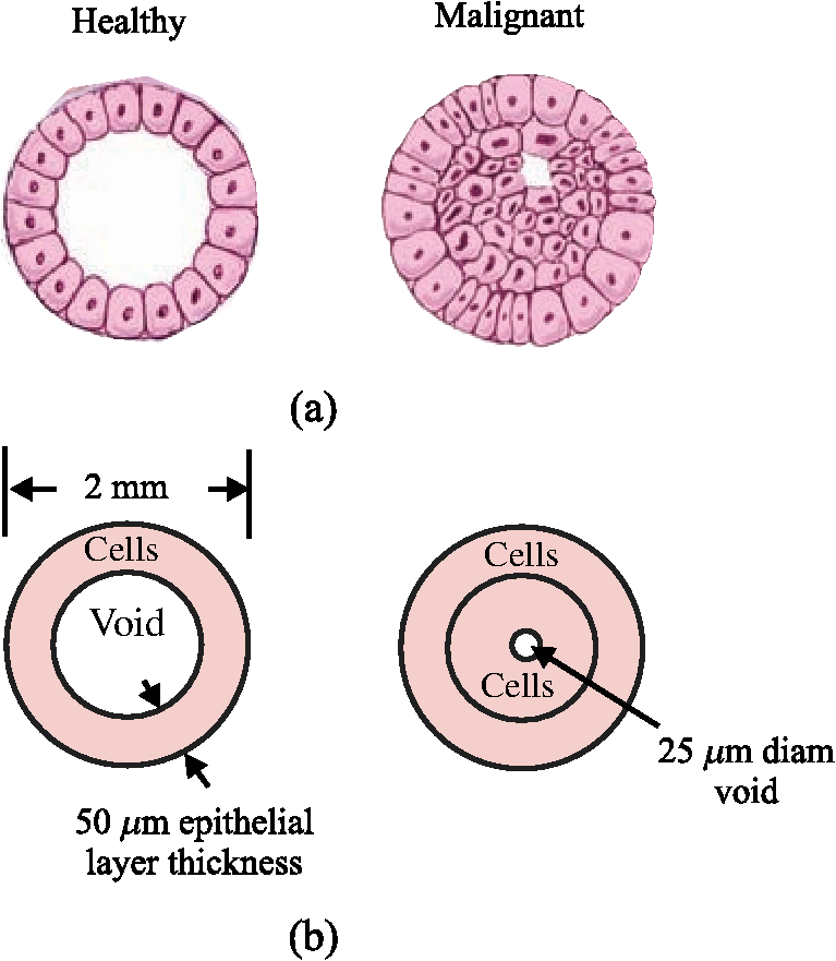

2.1.2.

Epithelial cell

An epithelial cell of $20\text{-}\mu \mathrm{m}$ diameter was assumed. Grover et al.⁴⁹ measured the density of a single cell using Archimede methods to be $1.08\mathrm{g}/{\mathrm{cm}}^3$. The epithelial cell of mass 4.524 ng was simplified by looking at all of its constituents as a combination of five basic categories: water, lipids, nucleic acids, proteins, and carbohydrates. The fractional weights ($w$) were those estimated by Watson⁵⁰ for a typical active human cell and are shown in Table 1 along with corresponding masses. Let the DNA, RNA, proteins, and carbohydrates be collectively referred to as the other part of the epithelial cell (OTCell). The fractional volumes $\nu$ also shown in Table 1 for each group were estimated using densities $1.0\mathrm{g}/{\mathrm{cm}}^3$ for water and $0.93\mathrm{g}/{\mathrm{cm}}^3$ for fat. As a result, the OTCell’s density was estimated to be $1.40\mathrm{g}/{\mathrm{cm}}^3$. Here, we consider the lipids as fatty tissue. By making a few simple approximations as to the constituents of each of the five categories, one can determine the amount of carbon, oxygen, hydrogen, nitrogen, sulfur, and phosphorus that exists in an epithelial cell. The total number of hydrogen atoms in the 3.23 ng of water in the epithelial cell is given by

Eq. (2)

$$\#\text{Hydrogen atoms}=\frac{(2\mathrm{H}/\text{molecule})(3.23\mathrm{ng})N_{\mathrm{A}}}{(18\mathrm{g}/\mathrm{mol})}.$$

Table 1

The fractional masses,50 masses and fractional volumes of the groups in a typical active human cell.

Group	Fractional weight (w)	Mass (ng)	Fractional volume (ν)
Water	0.714	3.23	0.771
Lipids	0.02	0.0905	0.0232
DNA	0.01	0.0452	0.2058
RNA	0.068	0.308
Proteins	0.158	0.715
Carbohydrates	0.03	0.136

The number of oxygen atoms was calculated similarly and the results are given in Table 2.

Table 2

The total number of each of the predominant atoms found in the epithelial cell.

Category	C	O	H	N	P	S
Water	0	$1.08\times {10}^{14}$	$2.16\times {10}^{14}$	0	0	0
Lipids	$3.06\times {10}^{12}$	$5.56\times {10}^{11}$	$5.63\times {10}^{12}$	$6.96\times {10}^{10}$	$6.96\times {10}^{10}$	0
DNA	$7.86\times {10}^{11}$	$6.26\times {10}^{11}$	$1.11\times {10}^{12}$	$2.98\times {10}^{11}$	$8.07\times {10}^{10}$	0
RNA	$5.18\times {10}^{12}$	$4.38\times {10}^{12}$	$7.51\times {10}^{12}$	$2.02\times {10}^{12}$	$5.47\times {10}^{11}$	0
Proteins	$1.58\times {10}^{13}$	$8.76\times {10}^{12}$	$3.22\times {10}^{13}$	$4.56\times {10}^{12}$	0	$1.43\times {10}^{11}$
Carbohydrates	$2.72\times {10}^{12}$	$2.72\times {10}^{12}$	$5.44\times {10}^{12}$	0	0	0
Total	$2.75\times {10}^{13}$	$1.25\times {10}^{14}$	$2.68\times {10}^{14}$	$6.95\times {10}^{12}$	$6.97\times {10}^{11}$	$1.43\times {10}^{11}$

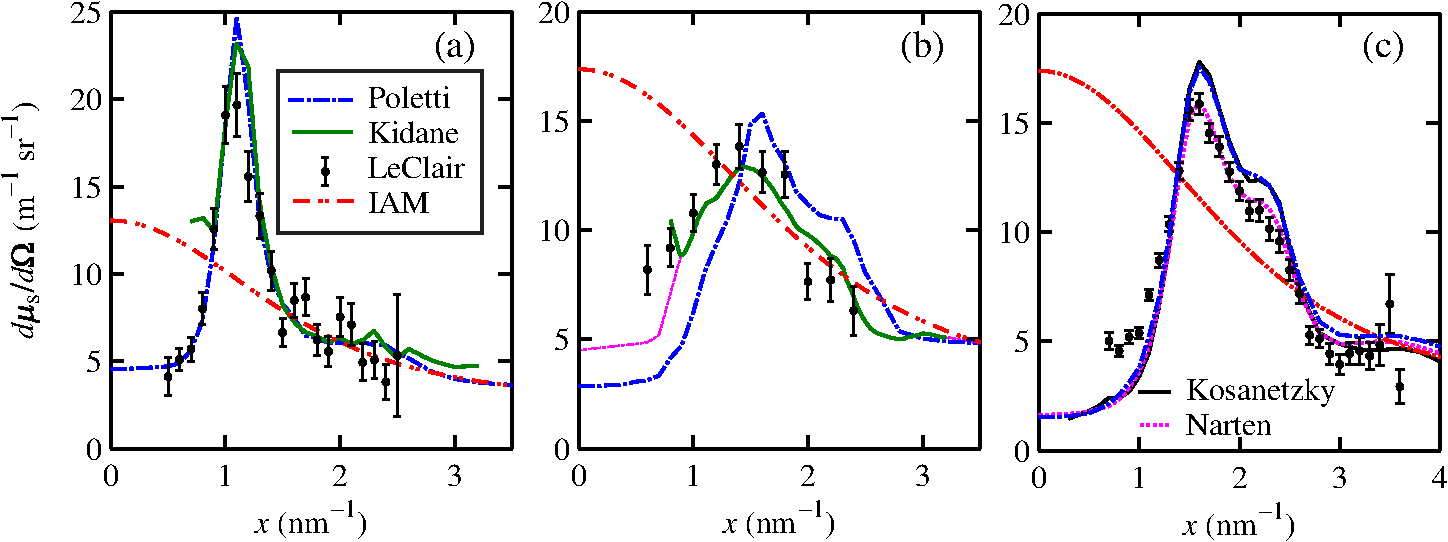
The majority of lipids in mammalian cells are found in the cell membrane to allow for elasticity and protection from foreign bodies. Lipids in the cell membrane are primarily referred to as phospholipids. Phosphatidylcholine, which has a molecular formula of ${\mathrm{C}}_{44}{\mathrm{H}}_{81}{\mathrm{O}}_8\mathrm{NP}$ and a molar mass of $783\mathrm{g}/\mathrm{mol}$, is the most common one. Table 2 shows the amount of carbon, oxygen, hydrogen, nitrogen, and phosphorus found within the lipid category of the epithelial cell.

Nucleic acids are the building blocks of the genetic information found within the cell’s nucleus, and they make up two distinct structures: deoxyribonucleic acid (DNA) and ribonucleic acid (RNA). In total, there are five different nucleic acids: adenine, thymine, guanine, cytosine, and uracil. In both DNA and RNA, these nucleic acids are linked in a chain by nucleoside monophosphate groups. A subunit in DNA and RNA can be thought of as a nucleic acid joined to a nucleoside monophosphate group, both of which have a known chemical formula. The nucleic acid component of the cell has elements: carbon, oxygen, hydrogen, nitrogen, and phosphorus. However, there are slight differences between the DNA and RNA structures. DNA is composed of only adenine, guanine, cytosine, and thymine, whereas RNA is composed of adenine, guanine, cytosine, and uracil in replacement of thymine. Since there are four possible subunits found in either structure, the assumption was made that there is 25% of each subunit found in either DNA or RNA. The atom contents in both structures are summarized in Table 2.

Amino acids are the building blocks of all proteins. The amino acids are linked together to make a long protein chain. Each amino acid has a different chemical formula, as well as an average frequency of occurrence in proteins, which was found by Sanejouand and Trinquier⁵¹ when they analyzed 105,990 protein sequences in the nonredundant OWL protein database (release 26.0 e). Using the amino acid chemical formula and frequencies of occurrence allowed calculations of atom content shown in Table 2 for the protein portion of the epithelial cell.

Carbohydrates are essentially sugars that provide energy to the cell through the metabolic processes occurring within the mitochondria. The most common metabolic process by far is glycolysis, which is the breaking down of glucose to form the ATP complex, or adenosine triphosphate, which acts as the cell’s main source of energy. Thus, this makes the glucose the single most abundant carbohydrate found in growing cells. Glucose has a chemical formula of ${\mathrm{C}}_6{\mathrm{H}}_{12}{\mathrm{O}}_6$ and a molar mass of about $180\mathrm{g}/\mathrm{mol}$. The amount of carbon, oxygen, and hydrogen within the 0.136-ng carbohydrate portion of the epithelial cell is shown in Table 2.

2.1.3.

Biopsy

Consider biopsies of thicknesses from 2 to 20 mm contained within the shaft of a seven-gauge needle. Figure 2 shows a schematic of a section of a 2-mm diameter duct being pierced by the needle. The black circle represents a cross section of the needle’s 3.81-mm inner diameter. The duct is surrounded by fibroglandular (fib) tissue. There is also fib on top and below the duct, the amounts dictated by the thickness of the biopsy. A 2-mm diameter x-ray beam was assumed to enter at the top of the shaft and the WAXS from a 2-mm diameter cylindrical shaped region of interest (ROI) was calculated by the technique described later in Sec. 2.3. First, the modeling of the biopsy composition and source of input scatter cross-section data are presented.

Fig. 2

A region of interest (ROI) is highlighted on the duct biopsy (top view).

During a biopsy procedure, it was assumed that a healthy duct will compress, whereas a duct with DCIS will not compress appreciably because of the extra epithelial cells. The composition within the cylindrical shaped ROI was approximated as follows. For a biopsy of thickness $d$, the volume of the ROI is $V_{\mathrm{roi}}=\pi {(1\mathrm{mm})}^2\times d$, volume of the intersection of the 2-mm diameter nondiverging WAXS beam and 2-mm diameter duct is $V_{\mathrm{int}}=16/3\times 1{\mathrm{mm}}^3=5.33{\mathrm{mm}}^3$, and the volume of fib within the biopsy for an uncompressed duct is $\mathrm{\Delta }V=V_{\mathrm{roi}}-V_{\mathrm{int}}$. During a biopsy procedure of a healthy duct, it was assumed that the duct collapsed and its void replaced with fib tissue. The amount of this fib volume irradiated was $V_{\text{void}\to \mathrm{fib}}^{\mathrm{h}}=4.92{\mathrm{mm}}^3$. The volume of fib in the ROI of the biopsy for the WAXS simulations was $V_{\mathrm{fib}}^{\mathrm{h}}=\mathrm{\Delta }V+V_{\text{void}\to \mathrm{fib}}^{\mathrm{h}}$, whereas the remaining volume filled with epithelial cells was $V_{\text{cell}}^{\mathrm{h}}=V_{\mathrm{roi}}-V_{\mathrm{fib}}^{\mathrm{h}}=0.71{\mathrm{mm}}^3$. For the malignant duct biopsy, the $25\text{-}\mu \mathrm{m}$ diameter void was replaced with fib and the volume $V_{\text{void}\to \mathrm{fib}}^{\mathrm{m}}=9.82\times {10}^{-4}{\mathrm{mm}}^3$ represented the portion irradiated. The volume of fib in the ROI of the malignant biopsy was $V_{\mathrm{fib}}^{\mathrm{m}}=\mathrm{\Delta }V+V_{\text{void}\to \mathrm{fib}}^{\mathrm{m}}$ and $V_{\text{cell}}^{\mathrm{m}}=V_{\mathrm{roi}}-V_{\mathrm{fib}}^{\mathrm{m}}=5.36{\mathrm{mm}}^3$ was its epithelial cell volume. Although fat could be present during a biopsy procedure, a WAXS fat subtraction protocol^42,43 can be applied to eliminate the effects of fat.

The volumes were calculated based on intersections of cylinders; however, for the simulations, the biopsies consisted of a rectangular prism of cells embedded in a cylinder of fib tissue. For the malignant biopsy, the epithelial cell component was of thickness $d_{\text{cell}}^{\mathrm{m}}=V_{\text{cell}}^{\mathrm{m}}/V_{\mathrm{ROI}}\times d=1.71\mathrm{mm}$, whereas it was $d_{\text{cell}}^{\mathrm{h}}=V_{\text{cell}}^{\mathrm{h}}/V_{\mathrm{ROI}}\times d=0.23\mathrm{mm}$ for the healthy one. The layer of epithelial cells was placed at three different positions within the column of fib: (i) its top surface at a depth of $d\times 0.1$, (ii) its center at the center of the column of tissue, and (iii) its bottom surface at $d\times 0.1$ from the column’s bottom. The three layered biopsies were subdivided into voxels. The cross section of each voxel was $0.1\times 0.1{\mathrm{mm}}^2$ and their depths were such that there were at least 10 voxels in depth for each layer.

2.2.

Scatter Cross Sections

The scatter cross-section data are important input variables to the model signal generator for predicting the potential use of scatter to diagnose malignant ducts. Figure 3 shows $d{\mu }_{\mathrm{s}}/d\mathrm{\Omega }$ evaluated at $\theta =6\mathrm{deg}$ for (a) breast fat, (b) fibroglandular tissue, and (c) water using different sources of data. In Fig. 3(a), both measured data by Kidane et al.⁴¹ and LeClair et al.³⁷ matched well with the data calculated using Poletti et al.⁴⁰ $F$ and Hubbell et al.⁵² $S$ values. Figure 3(b) shows data for fibroglandular tissue. The Poletti fib data are higher than those of LeClair and Kidane for $(1.5<x<2.7){\mathrm{nm}}^{-1}$. In Fig. 3(c) are shown the water data (i) measured by LeClair et al.,³⁷ (ii) calculated using Narten⁵³ $F$ and Hubbell et al.⁵² $S$, (iii) extracted from Kosanetzky et al.⁵⁴ data, and (iv) calculated using Poletti et al.⁴⁰ $F$ and Hubbell et al.⁵² $S$. The plot shows two groups obtaining different water signals for $(1.5<x<2.4){\mathrm{nm}}^{-1}$, namely, the Kosanetzky and Poletti data were higher than the LeClair and Narten data. The LeClair and Narten data were obtained quite differently, whereas Kosanetzky and Poletti used the independent atomic model (IAM) approximation at high $x$ to scale their data. The IAM data are also shown in Fig. 3. For the model predictions, the following $F$ data will be used: Poletti et al.⁴⁰ for fat, Narten⁵³ for water, and $F$ fib data extracted from Kidane et al.⁴¹ $d{\mu }_{\mathrm{s}}/d\mathrm{\Omega }$ data. The $d{\mu }_{\mathrm{s}}/d\mathrm{\Omega }$ data were extended to higher $x$ via the IAM and points were modified and added for $x<0.8{\mathrm{nm}}^{-1}$ [see Fig. 3(b), dashed line] by judging what happens for the case of fat [see Fig. 3(a)].

Fig. 3

$d{\mu }_{\mathrm{s}}/d\mathrm{\Omega }$ at $\theta =6\mathrm{deg}$ for (a) breast fat, (b) fibroglandular tissue, and (c) water.

The differential linear scattering coefficient of the epithelial cell was approximated by

Eq. (3)

$${\left(\frac{d{\mu }_{\mathrm{s}}}{d\mathrm{\Omega }}\right)}_{\text{cell}}={\nu }_{\text{water}}{\left(\frac{d{\mu }_{\mathrm{s}}}{d\mathrm{\Omega }}\right)}_{\text{water}}+{\nu }_{\text{lipid}}{\left(\frac{d{\mu }_{\mathrm{s}}}{d\mathrm{\Omega }}\right)}_{\text{fat}}+{\nu }_{\mathrm{OTCell}}{\left(\frac{d{\mu }_{\mathrm{s}}}{d\mathrm{\Omega }}\right)}_{\mathrm{OTCell}},$$

a weighted sum of $d{\mu }_{\mathrm{s}}/d\mathrm{\Omega }$ coefficients for water, fat, and the other constituents of the epithelial cell. The $F$ and $S$ data used in this work are shown, respectively, in Figs. 4(a) and 4(b). $F$ is in units of ${[\text{free electron per molecular weight}(W)]}^{0.5}$ and $S$ in (free electron per $W$). The $F$ for OTCell was calculated via the IAM (see Ref. 55 for a calculation example using ${\mathrm{H}}_2\mathrm{O}$) and $S$ for compounds using data for elements from Hubbell et al.⁵² Compositions for breast tissue were those measured by Poletti et al.⁴⁰ Figure 5(a) shows $d{\mu }_{\mathrm{s}}/d\mathrm{\Omega }$ at $\theta =6\mathrm{deg}$ for fibroglandular and the epithelial cell. The energies $E$ used were those indicated on the top energy axis. The epithelial cells are predicted to have a higher $d{\mu }_{\mathrm{s}}/d\mathrm{\Omega }$ than fib for $(0\le x<0.7428){\mathrm{nm}}^{-1}$ (region 1) and $x>1.39{\mathrm{nm}}^{-1}$ (region 3), whereas in region 2, the opposite occurred. Due to the IAM use at low $x$ for the OTCell, the $d{\mu }_{\mathrm{s}}/d\mathrm{\Omega }$ for the epithelial cell has a slow monotonic increase as $x\to 0$. Although the scatter data for both fib and the epithelial cells for $x<0.8{\mathrm{nm}}^{-1}$ were questionable, the range was included in the study. The main findings would not change if one was to exclude the range since regions 2 and 3 would provide sufficient contrast.

Fig. 4

Scattering coefficients: (a) $F$ and (b) $S$ for fat, fib, water, and the other component of the cell (OTCell).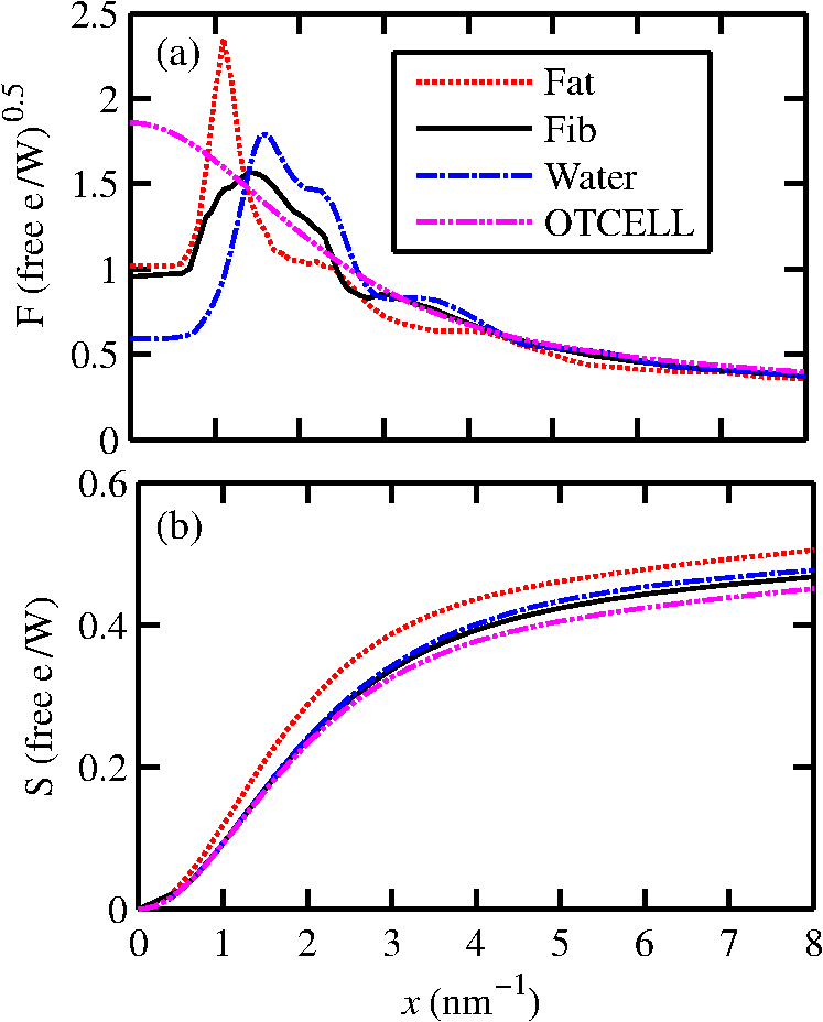

Fig. 5

Scattering coefficients: (a) $d{\mu }_{\mathrm{s}}/d\mathrm{\Omega }$ at $\theta =6\mathrm{deg}$ for fib and the epithelial cell and (b) $\mu$ values for tissue, OTCell, water, and the epithelial cell.

For the calculations of the scatter signals, $\mu$ values shown in Fig. 5(b) were used. The $\mu$ data for breast tissue were taken from Ref. 1, water and OTCell $\mu$ were obtained using the mixture rule and cross-section data from Plechaty et al.,⁵⁶ and the $\mu$ for the epithelial cell was estimated by

Eq. (4)

$${\mu }_{\text{cell}}(E)={\nu }_{\text{water}}{\mu }_{\text{water}}(E)+{\nu }_{\text{lipid}}{\mu }_{\text{fat}}(E)+{\nu }_{\mathrm{OTCell}}{\mu }_{\mathrm{OTCell}}(E).$$

2.3.

Signal Generator

For the simulations, a 2-mm diameter nondiverging 110-kV 2.5-mm Al filtered⁵⁷ beam entered the shaft of a seven gauge needle to interact with the duct biopsy which ranged from $d=2$- to 20-mm thick. The distance between the bottom of the biopsy and a flat matrix of CZT detector pixels was fixed at 40 cm. Figure 6, a scatter geometry schematic, will aid in describing how the calculations of $N_{\mathrm{s}}$ on the detector plane were computed. Since the single scatter field is circular symmetric about the primary beam, the signals in 11 annuli $(\mathrm{\Delta }\theta =1\mathrm{deg})$ centered at angles 3, 4, …, and 13 deg were calculated. These angles were defined with respect to the center of the biopsy. An enforced condition was that the single scattered photons contributing to a given annulus must have exited through the open bottom of the needle. As the biopsy thickness increases, the number of annuli that can be used to form the signal reduces because of this requirement. For example, for the 20-mm thick biopsy, only the $\theta =2\mathrm{deg}$ annulus can be used. Each annulus was divided into two subrings such that their widths (i.e., radial distance on detector plane) were $\approx 3\mathrm{mm}$. These subrings were then subdivided into pixels of an area each $dA\approx 9{\mathrm{mm}}^2$. Consider a pixel $\eta$ in a subring of the annulus $\theta$. The number of scattered photons each of energy $E$ in pixel $\eta$ due to voxel $k$ was approximated by

Eq. (5)

$$N_{\mathrm{s},\eta }^k(E,\theta )=N_0^k(E)\hspace{0.17em}{e}^{-\sum _i{\mu }_i(E){\mathrm{\Delta }}_i}\left[\frac{\frac{d{\mu }_{\mathrm{s}}^k[x(E,{\theta }_k)]}{d\mathrm{\Omega }}\frac{dA}{r_k^2}\cos {\theta }_k}{{\mu }_k(E)}\right]\left[\frac{(1-e^{-{\mu }_k(E){\mathrm{\Delta }}_k(1-\frac{1}{\cos {\theta }_k})})}{(1-\frac{1}{\cos {\theta }_k})}\right]\hspace{0.17em}{e}^{-\sum _j{\mu }_j(E)\frac{{\mathrm{\Delta }}_j}{\cos {\theta }_k}},$$

where $N_0^k(E)$ is number of incident photons of energy $E$ heading from the top of the biopsy to voxel $k$, $d{\mu }_{\mathrm{s}}^k/d\mathrm{\Omega }$ and ${\mu }_k$ are the scattering and total linear attenuation coefficients for tissue voxel $k$, ${\mathrm{\Delta }}_i$ is thickness of voxel $i$, ${\theta }_k$ is scatter angle for voxel $k$ and $r_k$ is distance from voxel $k$ to pixel $\eta$. The first exponential factor is responsible for attenuating the incident beamlet up to voxel $k$, whereas the second one attenuates the scattered photons from voxel $k$ that are heading toward pixel $\eta$. The first ratio in square brackets represents the probability of scattering toward pixel $\eta$ and the second one represents the fractional number of interactions in voxel $k$. The ($1-1/\cos {\theta }_k$) appears because scattering in voxel $k$ was assumed to take place along its central vertical axis all with angle ${\theta }_k$.^42,43

Fig. 6

Schematic of geometry showing some key parameters for the calculations of $N_{\mathrm{s}}$ (not to scale).

The total scatter count for energy $E$ within pixel $\eta$ due to all voxels $k$ is given by

Eq. (6)

$$N_{\mathrm{s},\eta }(E,\theta )=\sum _k{N}_{\mathrm{s},\eta }^k(E,\theta ).$$

Because of the symmetry of the phantoms, the signal of pixel $\eta$ was multiplied by the number of pixels in the subring to generate the total signal for the subring. Let $N_{\mathrm{s}}(E,\theta )$ correspond to the sum of all pixels within annulus $\theta$. The $N_{\mathrm{s}}(E,\theta )$ over all rings were then binned in terms of $x$ to obtain $N_{\mathrm{s}}^{\mathrm{H}}(x)\pm \sqrt{N_{\mathrm{s}}^{\mathrm{H}}(x)}$ and $N_{\mathrm{s}}^{\mathrm{M}}(x)\pm \sqrt{N_{\mathrm{s}}^{\mathrm{M}}(x)}$ for, respectively, the healthy and malignant duct biopsies. The angle used in the calculation of $x$ was the angle of the annulus in which the pixel was found.

The diagnostic signals for the healthy duct biopsies were given by

Eq. (7)

$$S_{\mathrm{H}}=S_1^{\mathrm{H}}-S_2^{\mathrm{H}},$$

where

Eq. (8)

$$S_1^{\mathrm{H}}=\sum _{x_n}{N}_{\mathrm{s}}^{\mathrm{H}}(x_n)\mathrm{and}{S}_2^{\mathrm{H}}=\sum _{x_m}{N}_{\mathrm{s}}^{\mathrm{H}}(x_m).$$

for $x_n$ values, where $N_{\mathrm{s}}^{\mathrm{H}}(x_n)+2\sqrt{N_{\mathrm{s}}^{\mathrm{H}}(x)}<N_{\mathrm{s}}^{\mathrm{M}}(x_n)-2\sqrt{N_{\mathrm{s}}^{\mathrm{M}}(x)}$ and $x_m$ where $N_{\mathrm{s}}^{\mathrm{H}}(x_m)-2\sqrt{N_{\mathrm{s}}^{\mathrm{H}}(x)}>N_{\mathrm{s}}^{\mathrm{M}}(x_m)+2\sqrt{N_{\mathrm{s}}^{\mathrm{M}}(x)}$. These so-called Poisson conditions incorporated the effects of Poisson noise and eliminated signals, which were too close. The conditions for allowed $x_n$ and $x_m$ needed to be satisfied for each of the three biopsy configurations simultaneously. Propagation of Poisson noise yielded a standard deviation for $S_{\mathrm{H}}$ given by

Eq. (9)

$${\sigma }_{S_{\mathrm{H}}}=\sqrt{S_1^{\mathrm{H}}+S_2^{\mathrm{H}}}.$$

Similarly, the malignant signal was given by

Eq. (10)

$$S_{\mathrm{M}}=S_1^{\mathrm{M}}-S_2^{\mathrm{M}},$$

where

Eq. (11)

$$S_1^{\mathrm{M}}=\sum _{x_n}{N}_{\mathrm{s}}^{\mathrm{M}}(x_n)\mathrm{and}{S}_2^{\mathrm{M}}=\sum _{x_m}{N}_{\mathrm{s}}^{\mathrm{M}}(x_m).$$

Using $S_{\mathrm{H}}$ and $S_{\mathrm{M}}$ as means and their associated ${\sigma }_{\mathrm{s}}$, Gaussian distributions $g_{\mathrm{H}}$ and $g_{\mathrm{M}}$ were generated and well separated ones could indicate a potential use of WAXS to diagnose malignancies in breast duct biopsies. For the biopsies with the epithelial cell layer at the center, the specificity

Eq. (12)

$$\mathrm{SPC}=\frac{\mathrm{TN}}{\mathrm{TN}+\mathrm{FP}},$$

and sensitivity

Eq. (13)

$$\mathrm{SES}=\frac{\mathrm{TP}}{\mathrm{TP}+\mathrm{FN}}$$

were computed for a decision threshold $t=(S_{\mathrm{H}}+S_{\mathrm{M}})/2$ and for $S_{\mathrm{M}}>S_{\mathrm{H}}$

Eq. (14)

$$\mathrm{TN}={\int }_{-\infty }^t{g}_{\mathrm{H}}(S)\mathrm{d}S,$$

Eq. (15)

$$\mathrm{FP}={\int }_t^{\infty }{g}_{\mathrm{H}}(S)\mathrm{d}S,$$

Eq. (16)

$$\mathrm{TP}={\int }_t^{\infty }{g}_{\mathrm{M}}(S)\mathrm{d}S,$$

Eq. (17)

$$\mathrm{FN}={\int }_{-\infty }^t{g}_{\mathrm{M}}(S)\mathrm{d}S.$$

Furthermore, if the $S_{\mathrm{H}}$ and $S_{\mathrm{M}}$ values among the biopsy configurations are similar, then this would suggest that the location of the duct within the biopsy need not be known.

The signal-to-noise ratio (SNR), defined by

Eq. (18)

$$\mathrm{SNR}=\frac{|S_{\mathrm{H}}-S_{\mathrm{M}}|}{\sqrt{{\sigma }_{S_{\mathrm{H}}}^2+{\sigma }_{S_{\mathrm{M}}}^2}},$$

was computed and a $\mathrm{SNR}>5$ would imply that the exposure time of 1 min could be reduced.⁵⁸ The study is meant to investigate the potential use of WAXS to diagnose malignancy independent of the detector response effects. The detector was assumed ideal (i.e., detective quantum efficiency of unity) and pixels varied in shape but were all $\approx 9{\mathrm{mm}}^2$ in area. A hypothetical unknown biopsy type will undergo a virtual experiment and this data will be analyzed and compared to relevant predictions so as to identify the biopsy type.

3.

Results

3.1.

Predictions

Figure 7 shows the $N_{\mathrm{s}}(x)$ signals for both malignant and healthy biopsies of thicknesses 2 to 20 mm with the epithelial cell layer at the center of the columns of tissue. Only $N_{\mathrm{s}}(x)$ at $x$ where either Poisson condition was satisfied simultaneously for all three biopsy configurations are given. As the thickness of the biopsy increases, there are less values of $x$ that were available for calculating $S_{\mathrm{H}}\mathrm{and}{S}_{\mathrm{M}}$ since fewer annular rings were involved. The thickness and associated angular ranges are given in each panel. The vertical dashed lines indicate the boundaries for the three regions that were identified in Fig. 5(a). In regions 1 and 3 (outer ones), the scatter signals of malignant biopsies (M-diamonds) were higher than those of healthy ones (H-triangles), whereas the opposite occurred in region 2 (i.e., H-squares $>\mathrm{M}$ circles). The number of points satisfying the conditions is indicated in each panel by the numbers in the first two parentheses (e.g., for the 2-mm biopsy, 29 points where M-diamonds $>\mathrm{H}$-triangles and 3 points where H-squares $>\mathrm{M}$-circles). From these data, the $S_{\mathrm{M}}$ and $S_{\mathrm{H}}$ signals shown in Fig. 8 were obtained. The error bars are shown yet they were smaller than the symbols. None of the signals between malignant and healthy overlap for a $1\sigma$ uncertainty. Note for $d>10\mathrm{mm}$, both $S_{\mathrm{H}}\mathrm{and}{S}_{\mathrm{M}}$ become negative.

Fig. 7

$N_{\mathrm{s}}(x)$ signals used to calculate the diagnostic signals for biopsy thicknesses ranging from 2 to 20 mm.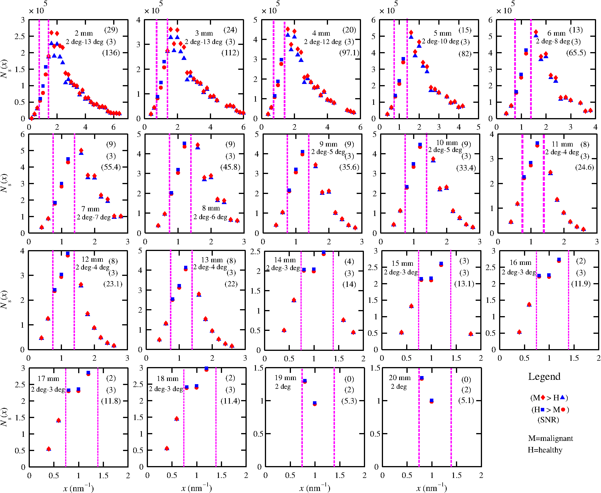

Fig. 8

$S_{\mathrm{M}}$ and $S_{\mathrm{H}}$ as a function of biopsy thickness.

The SNR values given between the third parentheses in each panel of Fig. 7 ranged from 136 (2 mm) to 5.1 (20 mm). For cases where the SNR is much $>5$, the 1-min exposure could be reduced. The $\mathrm{SPC}=\mathrm{SES}=1$ for all biopsy thicknesses and a receiver operating characteristic curve would have false positive rates $(\mathrm{FPR})=0$ for all true positive rates (TPR) and TPRs of unity for all FPRs. Calculations only took into account photon-quantum noise and as explained in Secs. 3.2 and 4 challenges do exist. However, first signals obtained for the different epithelial cell layer locations were compared.

The Gaussian probability distribution functions $g_{\mathrm{H}}$ and $g_{\mathrm{M}}$ for the three epithelial cell layer locations are shown in Fig. 9 for the (a) 15-mm and (b) 20-mm-thick biopsies. Now, suppose the threshold was set as above [i.e., $t=(S_{\mathrm{H}}+S_{\mathrm{M}})/2$ for the epithelial cell layer located at the center] yielding the vertical dashed lines for the 15- and 20-mm biopsies. For the 15-mm biopsies, the SPC and SES would maintain unity regardless of the location of the duct, whereas the SES reduced to 0.979 for a duct located at the top of the 20-mm-thick biopsy. Similarly, for biopsies of thicknesses $<19\mathrm{mm}$, the $\mathrm{SPC}=\mathrm{SES}=1$ regardless of where the epithelial cell layer was located. The results suggest that the detection of WAXS signals could be used to diagnose malignancy in breast duct biopsies. WAXS experimental measurements on a breast duct biopsy can be used in conjunction with the predictions for determining whether malignancy is present. A hypothetical experimental diagnostic task is described next.

Fig. 9

$S_{\mathrm{H}}$ and $S_{\mathrm{M}}$ Gaussian distributions for the (a) 15-mm and (b) 20-mm thick biopsies with the epithelial cell layer located at the three different positions: top, middle, and bottom of the biopsy.

3.2.

Hypothetical Experimental Diagnostic Task

Suppose interrogation of an 8-mm-thick breast biopsy containing a 2-mm diameter malignant duct at its center. Consider the stepwise data for obtaining the $S_{\mathrm{H}}$ and $S_{\mathrm{M}}$ diagnostic signals. Annuli from 2 to 6 deg were used to capture the scatter signals and each annulus was divided into two rings. The number of pixels in the inner and outer rings of the 4 deg annulus was 65 and 74, respectively. Figure 10(a) shows the $N_{\mathrm{s},\eta }(E,\theta =4\mathrm{deg})$ data in 5-keV increments for pixel $\eta$ located in the inner ring of the 4-deg annulus. The error bars represent Poisson noise, namely $\sigma =\sqrt{N_{\mathrm{s}}(E)}$. The count rates of $83.5\text{counts}/\mathrm{s}/\text{pixel}$ for both healthy and malignant biopsies can easily be processed by CZT flat panel detectors.⁵⁹ Evidently, trying to distinguish malignant from benign duct biopsies with a single pixel cannot be accomplished because of the noise. Instead, one needs to add the signals from many pixels and propagate the noise accordingly. The scatter signal in the $j$’th pixel of a ring within annulus $\theta$ was generated via

Eq. (19)

$$N_{\mathrm{s},\mathrm{j}}(E,\theta )=\mathrm{randn}\times \sqrt{N_{\mathrm{s},\eta }(E,\theta )}+N_{\mathrm{s},\eta }(E,\theta ),$$

where randn is a psuedorandom scalar drawn from the standard normal distribution. Figure 10(b) shows for photons with $E=60\mathrm{keV}$, the $N_{\mathrm{s}}$ values for the inner ring pixels. The $N_{\mathrm{s}}(E)$ signals obtained over all pixels in the 4-deg annulus were then added to yield $N_{\mathrm{s}}(E,\theta =4\mathrm{deg})$, which are shown in Fig. 10(c), for every 5-keV increment. The error bars were smaller than the symbols used to plot the data. Adding the signals and the noise in quadrature reduced uncertainties. The top axis corresponds to the $x$ values, which were calculated for this particular ring by using $\theta =4\mathrm{deg}$. The vertical dashed lines represent the values of $x$ for defining the three regions that were shown in Fig. 5(a). The mean of the angles used in the calculations of $N_{\mathrm{s}}$ for the malignant biopsy were $3.751\mathrm{deg}\pm 0.074\mathrm{deg}$ (inner ring) and $4.251\mathrm{deg}\pm 0.074\mathrm{deg}$ (outer). There are differences between the healthy and malignant biopsy cases for this particular annulus. However, to increase the diagnostic signals, the data from all annuli were similarly calculated and then binned in terms of $x$, as was done in Sec. 3.1.

Fig. 10

Data for the 8-mm thick healthy and malignant biopsies with the epithelial cell layer at the center: (a) $N_{\mathrm{s},\eta }(E,4\mathrm{deg})$ for pixel $\eta$ located in the inner ring of 4-deg annulus, (b) $N_{\mathrm{s}}(E=60\mathrm{keV})$ as a function of pixel $j$ in inner ring of 4-deg annulus, and (c) $N_{\mathrm{s}}(E,\theta =4\mathrm{deg})$.

The Gaussian distributions shown in Figs. 11(a)–11(c) are all the same and correspond to the predictions of $S_{\mathrm{M}}$ and $S_{\mathrm{H}}$ distributions for the 8-mm-thick biopsies. The values of $x$ used in the calculations were those corresponding to the 8-mm-thick biopsy in Fig. 7. The decision threshold shown was as before the mean of both values. The arrows in panels (a) and (b), respectively, correspond to malignant and healthy signals for other biopsy thicknesses, whereas in (c), they represent the malignant signals of 8-mm-thick biopsies with different malignant epithelial cell layer thicknesses. For generating all signals denoted by arrows, the same values of $x$ as for the 8-mm-thick biopsy were used. From Fig. 11(a), one can say that an unknown biopsy erroneously estimated to be 8-mm-thick would be diagnosed correctly if its actual thickness was $\ge 7.3\mathrm{mm}$. Similarly, Fig. 11(b) implies that a healthy biopsy estimated to be 8-mm-thick would be diagnosed correctly if its thickness was $\le 8.7\mathrm{mm}$. Therefore, to safeguard against false positives or false negatives, the thickness of the unknown biopsy erroneously estimated to be 8-mm thick would need to be between 7.3- and 8.7-mm thick. Figure 11(c) reveals that an 8-mm thick malignant duct biopsy would be diagnosed correctly provided the malignant epithelial cell layer thickness $>0.96\mathrm{mm}$. Although a finer step size for the varying thicknesses and inclusion of Gaussian distributions for their signals would yield better limits, the findings here sufficed to provide rough estimates.

Fig. 11

Signals via arrows: (a) $S_{\mathrm{M}}$ and (b) $S_{\mathrm{H}}$ for biopsies ranging in thickness from 7.1 to 8.9 mm but erroneously labeled as 8-mm thick and (c) $S_{\mathrm{M}}$ for 8-mm-thick biopsies with different malignant epithelial cell layer thicknesses. The $S_{\mathrm{H}}$ and $S_{\mathrm{M}}$ Gaussian distributions were for 8-mm-thick biopsies and were calculated using the procedure in Sec. 3.1, whereas the “arrow” signals were generated using the same $x$ values but with noise incorporated into the pixels.

4.

Discussions

The predicted specificities and sensitivities of unity indicated a potential use of WAXS signals to diagnose DCIS in biopsies. The predictions were based on ideal conditions, such as knowledge of the incident spectrum, accurate scatter cross-section data, and no detector response issues. Although challenging, quantitative assessments of the key variables are possible.

The geometry can be easily determined while the incident spectrum $N_0$ can be estimated via an x-ray scatter technique.⁴² Although beam divergence was not included, it can be incorporated into the simulations. Given the small dimensions of the sample and the beam, the multiple scatter would be negligible and much of it would be absorbed in the needle. If multiple malignancies exist within the biopsy, then the signal obtained would be even further from the signal predicted for a healthy condition.

A custom built energy dispersive CdTe breast biopsy x-ray diffractometer^37,42,43 will be used to measure the WAXS signatures of breast tissue and of epithelial cells over a large range of $x$. Signals at lower $x$ where destructive interference occurs may yield some useful diagnostic contrast between fib and the epithelial cells. Although fat tissue within the biopsies was neglected for this analysis, it can be corrected via use of a WAXS fat subtraction protocol.^42,43 Although CZT or CdTe detectors are known to have problems with hole tailing and fluorescence escape, a detector response function model⁶⁰ can be used to correct the pixel signals.

Knowledge of the amount of tissue that has been extracted occurs once the biopsy has been extracted from the needle. Here, the WAXS signals for biopsies were predicted when the tissue was within the needle. Perhaps, needles constructed out of a translucent plastic would facilitate tissue thickness estimation. The analysis of using other gauge needles needs to be assessed and perhaps plastic ones would allow more of the detector pixels to be used for the larger biopsies. The effects of the needle wall and its shape at the bottom would be quantified.

A typical duct diameter of 2 mm found in Ref. 48 was used. For an 8-mm-thick biopsy, it was shown that the malignant epithelial cell layer thickness must be $>0.96\mathrm{mm}$ for proper diagnosis. CBCT could provide estimates of the duct diameters, biopsy thicknesses, and help estimate the presence of gaps. The presence of gaps can be incorporated into the model signal generator (e.g., a new smaller thickness could be estimated). In fact, the use of CBCT to locate the duct and determine whether malignancy is present may be feasible and could compliment this work. The application of CBCT for the visualization of cell clusters in breast biopsies was presented at SPIE Medical Imaging 2013: Physics of Medical Imaging.⁶¹ Results were interesting, yet the finite focal spot size, which leads to geometric blur, was not evaluated.

5.

Conclusions

This work has shown that model predictions of the scatter signals from malignant versus healthy duct biopsies were sufficiently different so as to be of diagnostic use. Selectively adding signals according to their momentum transfer values provided a means to obtain useful signals. The preliminary findings encourage further efforts including an experimental study.