QuantitativeT2: interactive quantitative T2 MRI witnessed in mouse glioblastoma

Tonima Sumya Ali; Thorarin Albert Bjarnason; Donna L. Senger; Jeffrey F. Dunn; Jeffery T. Joseph; Joseph Ross Mitchell

doi:10.1117/1.JMI.2.3.036002

21 July 2015 QuantitativeT2: interactive quantitative T2 MRI witnessed in mouse glioblastoma

Tonima Sumya Ali, Thorarin Albert Bjarnason, Donna L. Senger, Jeffrey F. Dunn, Jeffery T. Joseph, Joseph Ross Mitchell

Author Affiliations +

Journal of Medical Imaging, Vol. 2, Issue 3, 036002 (July 2015). https://doi.org/10.1117/1.JMI.2.3.036002

Abstract

The aim of this study was to establish an advanced analytical platform for complex in vivo pathologies. We have developed a software program, QuantitativeT2, for voxel-based real-time quantitative T2 magnetic resonance imaging. We analyzed murine brain tumors to confirm feasibility of our method for neurological conditions. Anesthetized mice (with invasive gliomas, and controls) were imaged on a 9.4 Tesla scanner using a Carr–Purcell–Meiboom–Gill sequence. The multiecho T2 decays from axial brain slices were analyzed using QuantitativeT2. T2 distribution histograms demonstrated substantial characteristic differences between normal and pathological brain tissues. Voxel-based quantitative maps of tissue water fraction (WF) and geometric mean T2 (gmT2) revealed the heterogeneous alterations to water compartmentalization caused by pathology. The numeric distribution of WF and gmT2 indicated the extent of tumor infiltration. Relative evaluations between in vivo scans and ex vivo histology indicated that the T2s between 30 and 150 ms were related to cellular density and the integrity of the extracellular matrix. Overall, QuantitativeT2 has demonstrated significant advancements in qT2 analysis with real-time operation. It is interactive with an intuitive workflow; can analyze data from many MR manufacturers; and is released as open-source code to encourage examination, improvement, and expansion of this method.

1. Introduction

The soft tissue contrast in magnetic resonance imaging (MRI) results from the water-filled biological microcompartments. Few MRI relaxation parameters, such as spin-lattice (T1) and spin-spin (T2) relaxation times, are designed to measure the distribution of water protons. T2 is specifically sensitive to the extent of water compartmentalization.¹ T2 times decrease as tissue water loses magnetization to surrounding molecules. For example, white matter (WM) has a short T2 time, compared to gray matter (GM) and cerebrospinal fluid (CSF), since WM water is highly compartmentalized by myelin bilayers that promote magnetization exchange. Consequently, it is possible to identify distinct pools of water molecules in biological tissues according to their unique T2 times. When pathological conditions induce changes in tissue structures, significant deviations from normal T2s may occur.

A two-dimensional T2-weighted MR image, which is commonly used in clinical practice, is created by taking a snapshot of the T2 decay for each voxel of the imaging plane. Quantitative T2 (qT2) imaging is more complex. It requires a Carr–Purcell–Meiboom–Gill (CPMG) imaging sequence² that applies multiple refocusing pulses to generate a multiecho T2 image. With sufficient data points, pure T2-weighted decays are computed and further analyzed to determine the combination of T2 times that contributed to the measured decay.³ This allows scientists to create T2 distributions and discern microcompartmental structures.⁴ Multiexponential T2 decay analysis has been applied to study cartilage,⁵ blood,⁶ muscle,⁷ fat,⁷ cervix,⁷ liver,⁸ breast,⁹ and prostate.¹⁰ In addition to medical applications, this method has been applied by food scientists to determine if cheese was made using raw or heat-treated milk,¹¹ and as a quality control tool for fat distributions in fried food.¹² In the brain, qT2 has been used to identify normal WM,¹³ GM,¹^,¹⁴ and tumor.¹⁵ This method has detected myelin content in multiple sclerosis¹⁶^,¹⁷ and uncovered previously undetected water compartments in human brain pathology in vivo.¹⁸^,¹⁹

The typical qT2 analysis proceeds as follows: (1) a multiecho T2 MR image is acquired; (2) a region of interest (ROI) is specified on the image; (3) decay data within the ROI are averaged; and (4) a T2 distribution is created by fitting a sum of weighted exponential decays to the averaged decay data.²⁰ To make the fit more resilient to noise, a regularization routine is often applied. Although qT2 showed promise for characterizing pathological structures, the following limitations have discouraged widespread clinical adoption of qT2. First, the placement of the ROI requires prior knowledge of where pathology is located. Second, the average signal of an ROI may mask important physiological variability of complex biological tissues. Third, the regularization causes underestimation of the myelin water fraction (MWF), and this error increases as the signal-to-noise ratio decreases.²⁰ Fourth, the analysis often requires multiple software programs with different interfaces and input requirements. The main objective of this study was to overcome these limitations and establish an advanced analytical platform for complex pathologies, in vivo.

For this purpose, we developed QuantitativeT2, an integrated tool for qT2 analysis. This new tool results from four novel contributions: (1) voxel-based multiexponential qT2; (2) voxel-based T2 distribution histograms; (3) interactive computation of quantitative parametric maps; and (4) numerical assessment of qT2 parameter maps for user-specified ROIs. We hypothesize that our method will improve the existing qT2 analysis. It should identify pathological tissues at early stages of disease with quantitative information on its progression. We analyzed an in vivo mouse model of human malignant glioma (MG) to assess its potentials. Diagnosis of MG is particularly challenging as it is diffuse, highly invasive, and patients rarely survive in the long-term.²¹ Animal MG models are commonly used to study the disease progression in a controlled environment. Although increased T2 times have been observed in mouse gliomas using conventional T2-weighted MRI, this method could not detect gliomas at early stages.²² Multiexponential T2 has been reported in rat glioblastoma,²³ but the contributing T2 values or underlying factors for multiexponential behavior were not explored. Our method allowed probing at the subvoxel level to quantify pathological T2 with specific information on tumor infiltration. We generated quantitative parametric maps that identified water compartment alterations caused by glioma invasion and compared these results to histology.

2. Materials and Methods

2.1.

Animal Model

The mouse MG model was established by implanting immunocompromised mice with patient-derived brain tumor initiating cells (BTICs), a subpopulation of brain tumor cells that maintain the ability to self-renew, proliferate, and give rise to differentiated daughter cells that repopulate the tumor.²⁴ BTICs, when implanted into the brains of severe combined immunodeficiency (SCID) mice, result in highly invasive tumors that closely resemble MG in humans.²¹^,²⁴^,²⁵ In this study, six-week-old female SCID mice (Charles River Laboratories, Ontario, Canada) were housed in groups of three and maintained on a 12-h light/dark schedule at a temperature of $22 \pm 1 ° C$ and a relative humidity of $50 \pm 5 %$ for a period of 14 weeks. Food and water were available ad libitum. For the experimental group ( $n = 3$ , malignant glioma or MG group), the MG tumor model was established on day 3 by inoculating each mouse intracerebrally, in the right putamen with $1 \times 10^{4}$ BTICs collected from human surgical specimens. The control group ( $n = 3$ , control or C group) contained three, age-matched, normal SCID mice. All animal and human tissue protocols were reviewed and approved by University of Calgary Animal Care Committee.

2.2.

MRI Protocol

All mouse brains (C and MG groups) were scanned in vivo on day 93 following the BTIC inoculation. The MR imaging was carried out using a 9.4 Tesla (T) Bruker Avance system (Bruker, Billerica, Massachusetts). Four axial slices were imaged from each brain using a CPMG sequence. With a repetition time of 3000 ms, 128 echoes were collected with 5.5 ms echo spacing and 4 averages. The slices were 0.75 mm thick, covering a $1.92 {cm}^{2}$ field of view. The image matrix contained $128 \times 128$ pixels. Each pixel represented signals from a voxel of $0.15 \times 0.15 \times 0.75 mm$ volume. MR data were saved in raw data format (8 bit unsigned). For each animal, the MR slice containing the largest cross-section of the mouse brain was selected for further analysis.

2.3.

T2 Decay Analysis

Multiexponential decay analysis was carried out following well-described techniques²⁶^,²⁷ applied most recently by our group²⁰ for ROI-based analysis. Briefly, if one assumes that the T2 decay within a particular voxel is multiexponential, and can be decomposed into a summation of monoexponential functions, then the signal, $y$ , measured at each of $N$ CPMG echoes can be modeled as

Eq. (1)

y_{i} = \sum_{j = 1}^{M} s_{j} \exp (- t_{i} / T 2_{j}), i = 1,2, \dots, N,

where

t_{i}

are the CPMG echo times,

M

is the number of T2 bins used to model the T2 decay (described in a subsequent paragraph), and

s_{j}

are the relative weightings for each monoexponential function.

Contrary to the conventional practice, we solved this equation to determine individual $s_{j}$ weightings—once for each voxel in the MR slice. This intensive computation was executed in C language by representing Eq. (1) as an $N \times M$ matrix [with $N$ rows corresponding to the echo measurement times ( $t_{i}$ ) and $M$ columns corresponding to the T2 bins] as shown in Eq. (2). With preset T2 bins, the unknowns, $s_{j}$ , were solved using iterative non-negative least-square (NNLS) algorithm by minimizing error between the model and the measured echoes.

Eq. (2)

[\begin{matrix} A_{1,1} & A_{1,2} & \dots & A_{1, M - 1} & A_{1, M} \\ A_{2,1} & A_{2, M} \\ \dots & \dots & \dots & \dots & \dots \\ A_{N - 1,1} & A_{N - 1, M} \\ A_{N, 1} & A_{N, 2} & \dots & A_{N, M - 1} & A_{N, M} \end{matrix}] [\begin{matrix} s_{1} \\ s_{2} \\ \dots \\ s_{M - 1} \\ s_{M} \end{matrix}] = [\begin{matrix} y_{1} \\ y_{2} \\ \dots \\ y_{N - 1} \\ y_{N} \end{matrix}] .

In this study, the echo magnitude reached the noise floor at the 97th echo. Therefore, $N$ was set to 96 and echoes 97 to 128 were not used to avoid analysis artifacts that can be caused by the Rician noise floor.²⁸ In addition, $M = 120$ logarithmically spaced T2 bins ranging from 8.25 ms ( $1.5 \times$ shortest echo time) to 1056 ms ( $2 \times$ longest echo time) were used to model the T2 decay in each voxel. The $T 2 - s_{j}$ combinations for every voxel were stored independently as T2 distributions, and also summed together to create a T2 distribution histogram for the entire MR slice.

2.4.

Quantitative Parametric Mapping

A T2 distribution is evaluated by gmT2 and WF measures. The gmT2 is mean T2 time on a log scale.²⁹ The graphic user interface (GUI) of QuantitativeT2 is equipped with two slider bars that allowed selection of a T2 range in the T2 distribution histogram. For a range between $T 2_{low}$ and $T 2_{high}$ , gmT2 of each voxel for the cross-sectional image was calculated using the following formula:

Eq. (3)

gmT 2 = \exp (\sum_{T 2_{low}}^{T 2_{high}} s_{j} \log (T 2_{j}) / \sum_{T 2_{low}}^{T 2_{high}} s_{j}) .

The gmT2 values were arranged in a parametric map, superimposed on a gray-scale T2 scan and displayed on upper left panel (Figs. 1 and 2). WF value indicates the relative signal strength of a T2 range with respect to the entire T2 distribution.¹ QuantitativeT2 computed WF values individually for each voxel using the following formula:

Eq. (4)

WF = \sum_{T 2_{low}}^{T 2_{high}} area (s_{j}) / \sum_{T 2_{\min}}^{T 2_{\max}} area (s_{j}),

where

T 2_{low}

and

T 2_{high}

defined the selected T2 range, and

T 2_{min}

and

T 2_{max}

were the minimum and maximum T2 times in the T2 distribution histogram.

Area (s_{j})

referred to the T2 distribution histogram area, made up of discrete

s_{j}

weightings, between the defined T2 times. The WF map was then superimposed on a gray-scale T2 scan and displayed in upper right panel (Figs. 1 and 2). The gray-scale scans are used for anatomical reference. We implemented flexible color mapping and window/leveling algorithms for improved visualization. A sketch function was implemented for both parametric maps for the user to draw an arbitrary ROI for further analysis. A local T2 distribution histogram was computed from the T2 data only within the user-defined ROI. These distributions were scaled for display such that the area under the distribution curve was 1 and represented 100% of the signals.

Fig. 1

Analysis workflow of QuantitativeT2 for a control mouse brain C1. (Video 1) (MOV, 1.86 MB) [URI: http://dx.doi.org/10.1117/1.JMI.2.3.036002.1].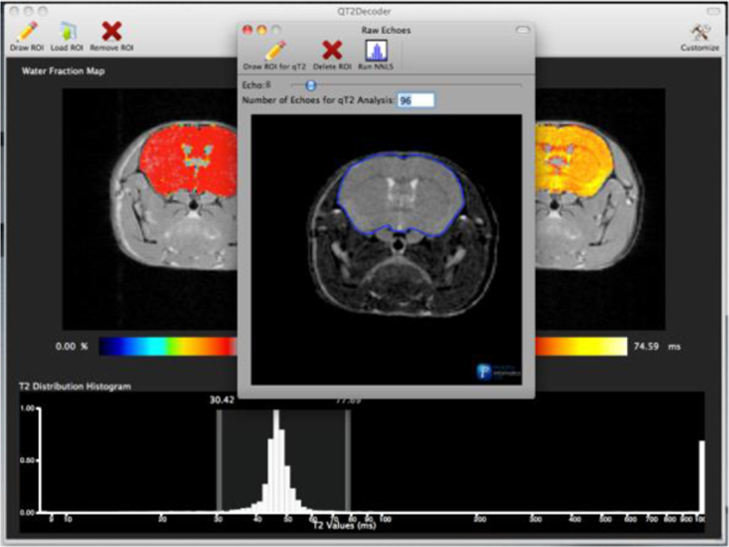

Fig. 2

Analysis workflow of QuantitativeT2 for a glioma induced mouse brain MG1. (Video 2) (MOV, 1.25 MB) [URI: http://dx.doi.org/10.1117/1.JMI.2.3.036002.2].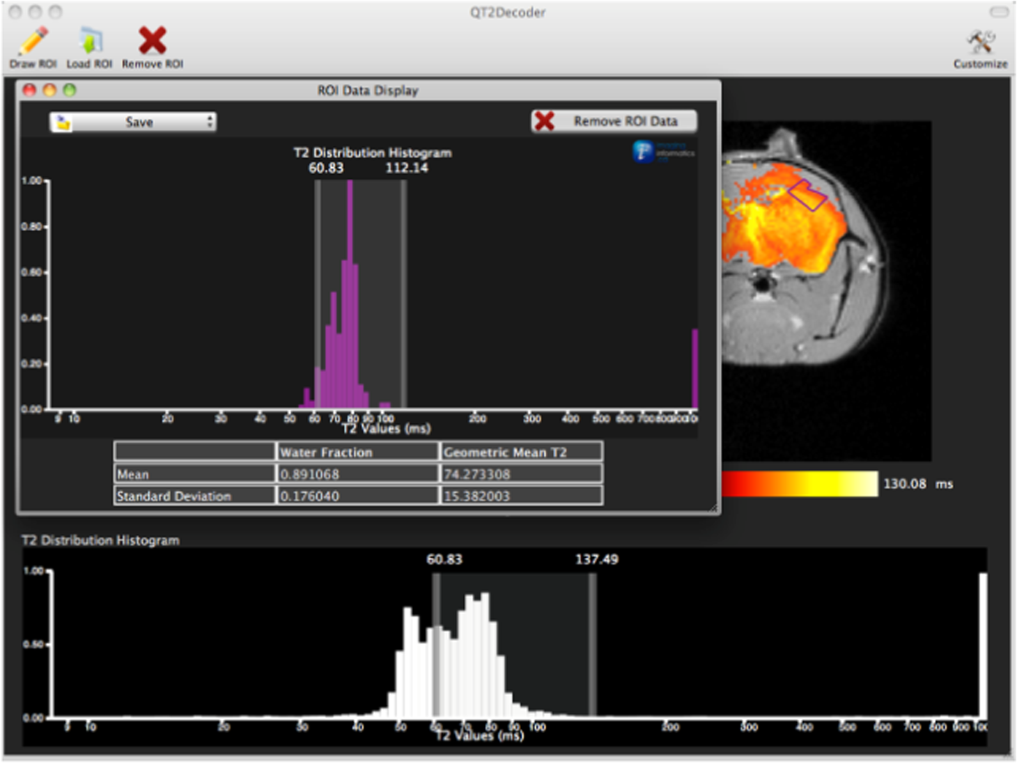

2.5.

Histological Analysis

The animals were immediately sacrificed following MRI. The brain from each animal was collected, fixed with 4% paraformaldehyde, paraffin-embedded, and cut into $5 - μ m$ -thick slices. For each mouse, a whole brain tissue section corresponding to the MR scan segment was stained for nestin, using an antibody against this human neural cell progenitor protein²⁵ (Sigma-Aldrich, Oakville, Ontario, Canada). Hematoxylin was used as a nuclear counter stain. A second tissue section within the MR scan slice was stained with hematoxylin and eosin (H&E) (EMD Chemicals, Gibbstown, USA; Sigma-Aldrich, Oakville, Ontario, Canada).

The quantitative analysis of the nestin stained histology sections was performed using the ACIS III automated cellular imaging system. It consisted of five steps: (1) the histology slide was digitized using ACIS III software; (2) the digital section was compared against the segmented gmT2 map of the same mouse, and histological regions corresponding to the T2 bands were identified; (3) within the histological region for each T2 band, four circular ROIs, each with a diameter of $500 μ m$ , were specified using ACIS III; (4) the percentage fraction of brown area (nestin stained, tumor cells) was calculated for each ROI; and (5) the average percentage was computed for the four ROIs corresponding to each T2 band. Data were collected from three control mice and three experimental mice by repeating the same process.

2.6.

QuantitativeT2 Architecture and Workflow

QuantitativeT2 was developed and tested on an Apple Mac Pro running Mac OS X 10.6. The Mac Pro was equipped with 3 GB of 1066 MHz DDR3 ECC SDRAM and powered by two 2.93 GHz Quad Core 45-nm Xeon W3540 processors. QuantitativeT2 used the C programming language for the computationally intensive voxel-based qT2 and the Objective C programming language for data management. The GUI was developed using Objective C and Interface Builder. The software components were organized according to the model view controller (MVC) architectural pattern and were compiled by Xcode (version 3.2). MVC isolated the application logic from data input and presentation. This allowed independent development and maintenance of the data processing and user interface units. Our matrix-fitting algorithm was written in the C programming language; it incorporated the open-source NNLS code developed and validated by Deguet.³⁰

Analysis in QuantitativeT2 followed a simple three-step approach. Step 1: the system performed voxel-based qT2 decay analysis for all voxels within the brain region. This produced a T2 distribution histogram, or a signature, that illustrated the general T2 properties of the tissue cross-section. The pathological T2 values may be visible in the distribution. Step 2: the user selected a T2 range from the histogram using slider bars. The system computed and displayed gmT2 and WF maps for the selected range in real time. These maps helped localize regions with pathological T2. Step 3: the user specified an ROI guided by the gmT2 map values and the extent of heterogeneity on the WF map. The mean and standard deviation of WF and gmT2 data within the ROI were then computed and saved.

3. Results

QuantitativeT2 has introduced a comprehensive voxel qT2 analysis method, by combining novel and existing features, which is intuitive and effective for disease diagnosis. Figure 3 shows proton density (PD) weighted and T2-weighted scans of C1 and MG1 as obtained from MR scanner. These scans are commonly used in clinical practice. Although informative, it is difficult to interpret these scans and isolate pathological tissues. Figures 1 and 2 show the analysis by QuantitativeT2 from raw MR data to parametric maps and numerical results for C1 and MG1.

Fig. 3

(a) Proton density weighted and (b) T2-weighted axial brain slice of control C1. (c) Proton density weighted and (d) T2-weighted axial brain slice of glioma induced MG1.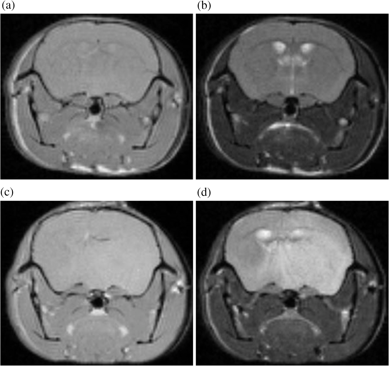

3.1.

T2 Distribution Histograms of C and MG Groups

Figure 4(a) displays the T2 distribution histogram computed from C1. Most of the signal was concentrated in a single peak centered at 47.6 ms with tightly packed values in the 30.4 to 60.8 ms range. A second peak corresponding to CSF was observed at 1056 ms. Figure 5(a) displays the T2 distribution histogram computed for MG1. The histogram was multimodal and shifted toward longer T2 compared to the histogram of C1. Three T2 peaks were observed centered at 51.7, 60.8, and 84.3 ms suggesting the presence of at least three different tissue types. A CSF peak was also observed at 1056 ms. For a comparison with control C1, the T2 values in this distribution were divided into two ranges: low (30.4 to 60.8 ms, same as C1) and high (63.4 to 149.2 ms, higher than C1).

Fig. 4

Quantitative T2 (qT2) analysis results of control C1 by QuantitativeT2. (a) The T2 distribution histogram for a single axial slice of C1, (b) the geometric mean T2 (gmT2) map, and (c) water fraction (WF) map computed for the T2 range 30.4 to 60.8 ms as specified in the histogram.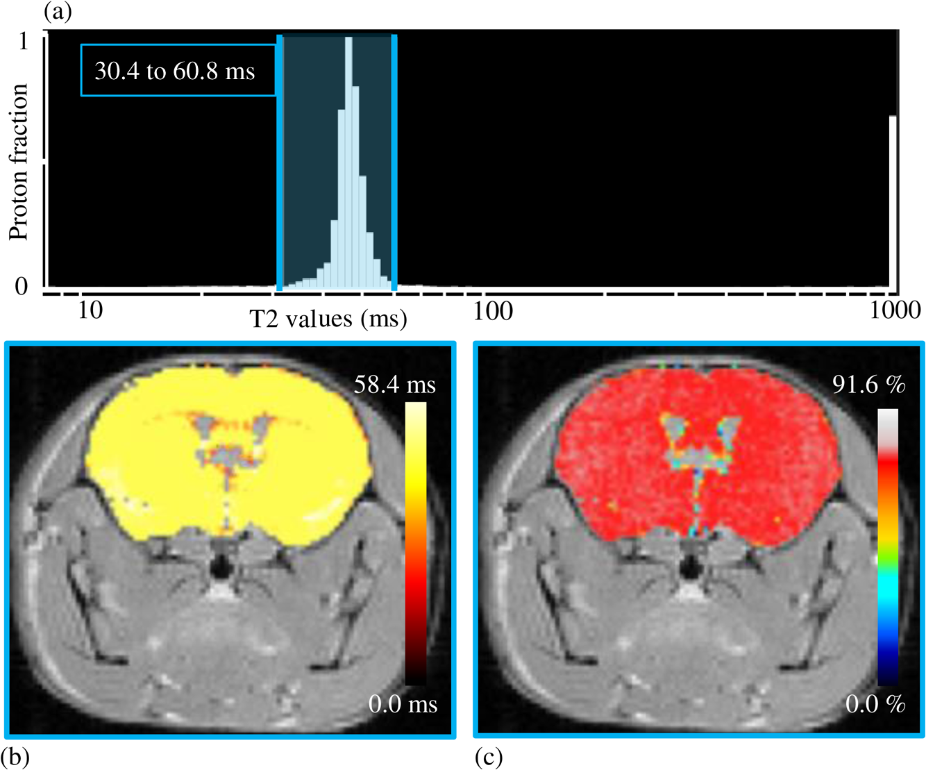

Fig. 5

(a) The T2 distribution histogram for a single axial slice of MG1. (b) The gmT2 map and (d) WF map computed for the T2 range of 30.4 to 60.8 ms outlined in blue. (c) The gmT2 map and (e) WF map highlighting the pathological tissues of the brain corresponding to the higher T2 range of 63.4 to 168.6 ms outlined in purple. (f) The local T2 distribution histogram from region of interest ROI drawn in (c) and (e). It is suggested that the ROI included multiple tissue types; gmT2 and WF measurements are shown. The last peak corresponds to cerebrospinal fluid.

3.2.

Tumor Segmentation by T2-Specific Mapping

Figures 4(b) and 4(c) display the gmT2 and the WF maps computed for the low T2s for mouse C1. The gmT2 map selectively displayed tissues corresponding to the T2 range specified in Fig. 4(a). It displayed the average T2 value, within the T2 range, for each voxel of the brain image according to Eq. (3). All the WM and GM tissues were highlighted in the map with gmT2 values in the 0 to 58.4 ms range, as shown by the color bar. The WF map in Fig. 4(c) also highlighted the brain tissues with T2 components in the 30.4 to 60.8 ms range, but with different information content. The color bar shows that the intensity of WF varied from 0.0 to 91.6% with a large number of pixels in the 70 to 85% range. For these pixels, the majority of signal strength came from the 30.4 to 60.8 ms range.

Figures 5(b) and 5(c) show the gmT2 maps computed for MG1. Only parts of the tumor-bearing mouse brain, the highlighted regions, were found to correspond to the first T2 range (30.4 to 60.8 ms, outlined in blue). The other parts of the brain corresponded to 63.4 to 168.6 ms, T2 values past the normal range of GM, as observed in Fig. 5(c). There, the gmT2 of the highlighted tissues were in the 0 to 149.2 ms range. These tissues were later found to contain tumor cells by histological analysis (see Sec. 3.5). Figures 5(d) and 5(f) display the WF maps generated for the same T2 ranges for MG1. Portions of the brain were highlighted for the T2 range of 30.4 to 60.8 ms with mostly homogeneous distribution [Fig. 5(d)]. Other regions of the brain corresponding to higher T2 values (outlined in purple) displayed a heterogeneous WF distribution in Fig. 5(e).

3.3.

Quantitative Characterization of Pathological Tissues

Figure 5(f) displays the local T2 distribution histogram computed from the ROI shown on the gmT2 and WF maps of MG1 [Figs. 5(c) and 5(e)]. The histogram showed a heterogeneous T2 distribution with two distinctive peaks. The first peak (51.7 to 71.6 ms) had a mean gmT2 of 65.8 ms with WF of 61.5%; and the second peak (74.6 to 99.2 ms) had a mean gmT2 of 78.7 ms with WF of 32.0%. The remaining 6.5% of the ROI signal corresponded to the CSF peak.

3.4.

T2-Based Segmentation of Normal and Pathological Tissues

Figures 6 and 7 show results from T2-based segmentation of normal and pathological tissues in the control (C1 to C3) and glioma (MG1 to MG3) groups, respectively. For each mouse brain, the following T2 ranges were defined in the T2 distribution histograms: T2 band 1: 30.4 to 60.8 ms, T2 band 2: 63.4 to 71.6 ms, T2 band 3: 74.6 to 84.3 ms, and T2 band 4: 87.8 to 149.2 ms. The gmT2 map of each mouse brain was segmented into four regions, one for each T2 band. These T2 bands and the corresponding regions are colored in cyan, maroon, red, and orange, respectively. ROIs were drawn individually for each segmented region for further analysis. Tables 1 and 2 summarize the gmT2 and the WF data for the control and the glioma group, respectively. These results demonstrate an alternative analysis method of QuantitativeT2.

Fig. 6

(a) to (c) Segmented T2 distribution histograms and corresponding gmT2 maps for controls C1 to C3. Each T2 distribution histogram is divided into four T2 bands: 30.0 to 60.8 ms (T2 band 1, cyan); 63.4 to 71.6 ms (T2 band 2, maroon); 74.6 to 84.3 ms (T2 band 3, red); and 87.8 to 149.2 ms (T2 band 4, orange). The gmT2 maps are segmented into four regions, one for each T2 band.

Fig. 7

(a) to (c) Segmented T2 distribution histograms and corresponding gmT2 maps for malignant glioma (MG) induced mouse brain scans, MG1 to MG3. Each T2 distribution histogram is divided into four T2 bands: 30.4 to 60.8 ms (T2 band 1, cyan); 63.4 to 71.6 ms (T2 band 2, maroon); 74.6 to 84.3 ms (T2 band 3, red); and 87.8 to 149.2 ms (T2 band 4, orange). The gmT2 maps are segmented into four regions, one for each T2 band.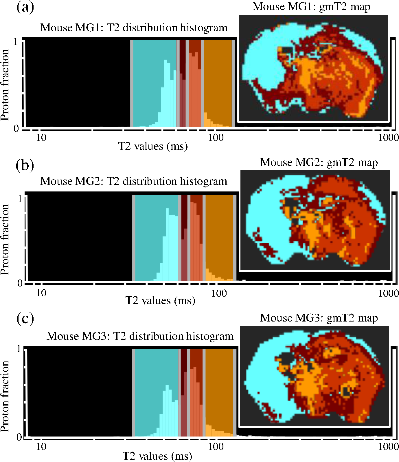

Table 1

The average geometric mean T2 (gmT2) and water fraction (WF) computed for two regions of interest (ROIs) corresponding to the first two T2 bands in the segmented T2 distribution histogram of controls C1 to C3 in Figs. 6(a)–6(c).

T2 band	Geometric mean T2 (ms)		Water fraction (%)
T2 band	1	2	1	2
ROI 1	$49.2 \pm 4.1$	$72.6 \pm 7.6$	$83.7 \pm 1.4$	$1.5 \pm 0.8$
ROI 2	$49.9 \pm 3.9$	$65.4 \pm 2.1$	$79.3 \pm 5.3$	$5.8 \pm 3.9$

Note: T2 band 1: 30.4 to 60.8 ms, corresponds to ROI 1. T2 band 2: 63.4 to 71.6 ms, corresponds to ROI 2.

Table 2

The average gmT2 and WF computed for four ROIs corresponding to the four T2 bands in segmented T2 distribution histograms of the malignant glioma (MG) induced mouse brain scans MG1 to MG3 in Figs. 7(a)–7(c).

T2 band	Geometric mean T2 (ms)				Water fraction (%)
T2 band	1	2	3	4	1	2	3	4
ROI 1	$52.1 \pm 0.7$	$67.4 \pm 1.1$	$74.6 \pm 5.1$	$100.1 \pm 11.4$	$68.8 \pm 1.7$	$9.7 \pm 2.3$	$6.2 \pm 1.3$	$2.4 \pm 1.6$
ROI 2	$57.3 \pm 1.1$	$67.5 \pm 0.6$	$77.7 \pm 1.3$	$92.2 \pm 3.4$	$22.7 \pm 5.5$	$47.9 \pm 9.8$	$17.2 \pm 3.1$	$2.5 \pm 1.6$
ROI 3	$60.6 \pm 1.4$	$69.2 \pm 0.3$	$78.4 \pm 0.4$	$92.2 \pm 3.7$	$4.5 \pm 3.5$	$28.9 \pm 5.1$	$49.9 \pm 11.9$	$7.4 \pm 4.6$
ROI 4	$59.9 \pm 0.4$	$69.1 \pm 1.0$	$78.2 \pm 0.7$	$103.9 \pm 5.0$	$1.2 \pm 0.9$	$20.2 \pm 9.5$	$23.0 \pm 12.5$	$39.2 \pm 10.1$

Note: T2 band 1: 30.4 to 60.8 ms; T2 band 2: 63.4 to 71.6 ms; T2 band 3: 74.6 to 84.3 ms; T2 band 4: 87.8 to 149.2 ms. ROIs 1 to 4 correspond to T2 bands 1 to 4.

3.5.

Comparison of qT2 with Histology

For validation purpose, the results obtained by QuantitativeT2 were compared against histology.

The histology stains of the control group C1 to C3 revealed no tumor cells (data not shown). Figure 8(a) shows that the four color-coded regions in the gmT2 map of the glioma-bearing mouse brain, MG1, correspond with varying tumor cell densities, when visually compared with Fig. 8(b). Here density of brown stain represents tumor cell population. At 40x magnification [Figs. 8(c)–8(f)], the increase in tumor cell population with increased T2 times is striking. The histological analysis also confirmed that the BTICs were initially implanted at the central mass of the pathological tissue (highlighted in orange in the gmT2 map). In Figs. 8(g)–8(j), the nuclei are stained blue and the extracellular matrix stained pink. Increasing tumor cell density was observed with the increase in T2 for the regions corresponding to T2 bands 1, 2, and 3. Degeneration of the extracellular matrix was observed in the regions corresponding to the highest T2 time, T2 band 4 [Fig. 8(j)]. Similar results were observed in brain sections stained for nestin or H&E from all three mice with glioma.

Fig. 8

Comparative analysis of qT2 results and histology for MG-induced brain slice. (a) The color-coded T2 distribution histogram and the corresponding segmented gmT2 map of MG1. The T2 bands are 30.4 to 60.8 ms (cyan); 63.4 to 71.6 ms (maroon); 74.6 to 84.3 ms (red); and 87.8 to 149.2 ms (orange). The T2 in the first band are normal values for gray matter, and the region colored in cyan indicates normal brain tissues. The other T2 bands hold increased T2 due to pathology and the corresponding regions indicate tumor tissues at different stages of development. (b) A histology section from the same magnetic resonance (MR) slice in mouse MG1 stained with an antibody for human nestin, where the density of brown stain indicates the tumor cell population. (c) to (f) Higher magnification (40×) images of the histological section corresponding to the four T2 bands: (c) shows normal tissue corresponding to cyan T2 band; (d) shows presence of tumor cells in tissue corresponding to maroon T2 band; (e) and (f) show increasing tumor cell population for red and orange T2 bands, respectively. (g) to (j) Higher magnification (40×) images of another histology section within MR scan slice stained with hematoxylin and eosin (H&E) from mouse MG1 corresponding to the four T2 bands: (g) shows tissue with few normal cells for cyan T2 band, (h) and (i) show increasing cell population for maroon and red T2 bands, respectively, and (j) shows increased cell population and extracellular matrix degradation. The cell nuclei are colored blue and the extracellular matrix is colored pink.

The histology sections stained for nestin were later quantified and analyzed using the ACIS III automated cellular imaging system for both control and tumor-bearing mice. For each whole brain section, histological regions corresponding to the T2 bands listed above were identified and the average percentages of brown area (tumor cell cytoplasm) were calculated for these regions. Figure 9 demonstrates the nestin stain percentages in normal brains for the control groups (C1 to C3) and BTIC tumor-bearing brains for the experimental group (MG1 to MG3). The T2 time increased, from 30.4 to 84.3 ms as the nestin stain% increased, and therefore, the tumor cell density increased. However, nestin% decreased in brain regions with the longest T2 times (87.8 to 149.2 ms). The data trends of nestin percentages were very strongly correlated ( $p < 0.001$ ) according to Spearman’s rank correlation coefficient³¹ among the MG tumor-bearing brains, MG1, MG2, and MG3.

Fig. 9

The nestin stain (brown area) percentages for the ROIs corresponding to four T2 bands: 34.0 to 60.8 ms; 63.4 to 71.6 ms; 74.6 to 84.3 ms; and 87.8 to 149.2 ms computed using ACIS III automated cellular imaging system. C1, C2, and C3 present data from normal mouse brains. These results are identical; the data from C1 and C2 are overlapped by the data from C3. MG1, MG2, and MG3 present data from the mouse brains with MG tumors. The T2 time increases, from 30.4 to 84.3 ms, as the nestin stain% increases, and therefore, the tumor cell density increases. However, nestin% decreases in brain regions with the longest T2 times (87.8 to 149.2 ms). H&E stains in these regions indicate they had degraded extracellular matrices compared to the other regions.

4. Discussion and Conclusion

Our voxel-based analysis method has enhanced the spatial resolution of qT2 analysis compared to ROI-based approaches. It now permits visual interpretation of the general T2 properties of all brain tissues in the scanned slice. Long T2 times are readily identified in the histogram, allowing easy localization of the corresponding anatomical regions. It has enabled the identification of T2 ranges of interest exhibiting subtle differences—these ranges would likely remain unidentified using the traditional ROI-based approaches. QuantitativeT2 has combined interactive computation and presentation of gmT2 and WF parametric maps. Two different properties—water microcompartment structure by gmT2 and partial voluming among these compartments by WF—are now revealed simultaneously by this arrangement. We have also improved the contrast and appearance of parametric maps by flexible color mapping and window leveling algorithms. The local ROI analysis tool has been effective for the isolation and characterization of specific tissues by gmT2 and WF measurements. Overall, we have improved the interpretation of qT2 results with a faster, easier, and intuitive workflow.

QuantitativeT2 is free and released as an open-source code. It can process the raw MR data from many manufacturers. It integrates mathematical processing, visual displays, and interactive analysis functionalities in one platform, such that no other software is required for data processing. It is also time-efficient; it completes qT2 analysis of $128 \times 128$ scan matrix in $< 2 s$ on a desktop/laptop computer running Mac OS X 10.6 or newer. Yoo et al. recently described a method for qT2 analysis that leveraged multicore CPU and graphical processing units to reduce computation time.³² Their work is highly complementary, and different from ours, in several important ways. Their work is geared toward rapid, noninteractive, batch processing of multiple exams and is focused on production of static MWF maps. Our tool is designed for a dynamic workflow and interactive mapping of gmT2 and WF.

In the literature, qT2 MRI has been shown effective for analyzing multiple neurological conditions, such as tumor,¹⁵ multiple sclerosis,¹⁶ and phenylketonuria.¹⁹ In the current study, we have analyzed MG, one of the most common primary central nervous system tumors in adults. In conventional MRI, a long T2 is observed in regions of increased tissue water and blood volume, as well as in areas where brain tissue texture has been lost from gliosis.³³ In a rat glioblastoma model, both short T2 ( $20.7 \pm 5.4 ms$ ) and long T2 ( $76.4 \pm 9.3 ms$ ) were observed in tumor ROIs, whereas a single T2 component ( $48.8 \pm 2.3 ms$ ) was observed for normal GM.²³ In the latter study, the ROI-based approaches used resulted in coarser spatial resolution and reduced detail in T2 histograms. In contrast, our voxel-based analysis method has shown that the T2 times between 30 and 150 ms are related to cellular density and the integrity of the extracellular matrix. The genotypic and phenotypic changes in MG are expected to result in high cellular density and matrix degeneration,³⁴ which is in accordance with our results. qT2 mapping has been recommended for improved monitoring of glioblastoma patients under therapy.³⁵ The analytical advancement from the conventional MRI to our analysis approach is clearly noticeable by comparing Fig. 3 with Fig. 5. The PD and T2 MRI in Fig. 3, which are applied in clinical settings, identify the pathological region but fail to isolate the tumor from normal tissues. Gray-scale intensity is the only information available for further diagnosis. For the same MR slice, voxel-based multiexponential MRI clearly delineates the tumor and provides quantitative information on tumor infiltration. The gmT2 and WF maps in Fig. 5 provide anatomical information specific to the progression of MG, which may assist in cancer staging. Likewise, QuantitativeT2 may also be useful for analyzing other neurological conditions and qT2 MRI data in general.

Due to technical constraints on data availability for human brain pathology, our method has been validated in a mouse model of MG up until the present date. The commonly used qT2 sequence scans one slice at a time, which is inadequate for patient screening. Currently available human qT2 data are acquired in research facilities and not clinical centers, which lack infrastructure to obtain the time-consuming multiecho sequences from all patients. Recently, promising progress has been made using new pulse sequences that accelerate multiecho data acquisition, while providing information from contiguous slices.³⁶^,³⁷ Combining the scans of multiple slices, these new sequences also produce significantly large data. The new pulse sequences may encourage the clinical application of qT2 only if there is an efficient analysis tool—QuantitativeT2—to process the data and visually integrate the qT2 analysis results. In fact, QuantitativeT2 has been validated against existing qT2 analysis methods and normal human data.³⁸

One limitation of MRI is its inherent low sensitivity level for identifying individual tumor cells. It can be argued that a very low concentration of tumor cells can remain unnoticed by voxel-based qT2 or T2-based segmentation as observed in the corpus callosum of the contralateral cerebral hemisphere in Fig. 8(b). This was due to the overwhelming effect of the normal tissue for a voxel volume ( $0.15 \times 0.15 \times 0.75 mm$ ). However, the heterogeneous WF map of this region in Fig. 5(b) shows $\sim 70$ to 80% of WF for the prominent tissue and highlights the importance of further analysis. Perhaps the quantitative ROI characterization [shown in Fig. 5(f)] would provide more information on the tumor cells in that region. The strong correlation among the MG data nestin percentages proves it beyond doubt that the MG tumor infiltration follows a unique behavior in all three mice presented here as shown in Fig. 9. The tumor infiltration is related to T2 alterations, which are detectable by voxel-based qT2 analysis, when the tumor cells are detectable within MRI hardware capacity.

In conclusion, we developed QuantitativeT2—a software package for simple and real-time voxel-based qT2 analysis. QuantitativeT2 brings significant advancement to existing qT2 MRI technology. It provides a novel and interactive workflow for identification and characterization of T2 distribution histograms along with gmT2 and WF parameter maps. With it, we identified structural changes in glioma progression in relation to T2 variations. Being open-source, QuantitativeT2 should promote the use of qT2 analysis in research as well as in diagnostics.

Acknowledgments

This project was funded by Alberta Innovates Health Solutions, Alberta Innovates Technology Futures, Alberta Cancer Foundation, and Southern Alberta Cancer Research Institute. Thanks to Mark Simpson and Jeff Packer for helpful advice and support for software development.

References

1.

K. P. Whittall et al., “In vivo measurement of T2 distributions and water contents in normal human brain,” Magn. Reson. Med., 37 (1), 34 –43 (1997). http://dx.doi.org/10.1002/mrm.1910370107 MRMEEN 0740-3194 Google Scholar

2.

S. Meiboom and D. Gill, “Modified spin-echo method for measuring nuclear relaxation times,” Rev. Sci. Instrum., 29 688 (1958). http://dx.doi.org/10.1063/1.1716296 RSINAK 0034-6748 Google Scholar

3.

K. P. Whittall, A. L. MacKay and D. K. B. Li, “Are mono-exponential fits to a few echoes sufficient to determine T2 relaxation for in vivo human brain?,” Magn. Reson. Med., 41 (6), 1255 –1257 (1999). http://dx.doi.org/10.1002/(SICI)1522-2594(199906)41:6<1255::AID-MRM23>3.0.CO;2-I MRMEEN 0740-3194 Google Scholar

4.

A. MacKay et al., “Insights into brain microstructure from the T2 distribution,” Magn. Reson. Imaging, 24 (4), 515 –525 (2006). http://dx.doi.org/10.1016/j.mri.2005.12.037 MRIMDQ 0730-725X Google Scholar

5.

L. Vidarsson et al., “Linear combination filtering for T2-selective imaging of the knee,” Magn. Reson. Med., 55 (5), 1191 –1196 (2006). http://dx.doi.org/10.1002/mrm.20878 MRMEEN 0740-3194 Google Scholar

6.

R. S. Menon and P. S. Allen, “Application of continuous relaxation time distributions to the fitting of data from model systems and excised tissue,” Magn. Reson. Med., 20 (2), 214 –227 (1991). http://dx.doi.org/10.1002/mrm.1910200205 MRMEEN 0740-3194 Google Scholar

7.

C. S. Poon and R. M. Henkelman, “Practical T2 quantitation for clinical applications,” J. Magn. Reson. Imaging, 2 (5), 541 –553 (1992). http://dx.doi.org/10.1002/jmri.1880020512 Google Scholar

8.

M. Lupu, C. D. Thomas and J. Mispelter, “Retrieving accurate relaxometric information from low signal-to-noise ratio 23Na MRI performed in vivo,” C. R. Chim., 11 (4–5), 515 –523 (2008). http://dx.doi.org/10.1016/j.crci.2007.09.007 Google Scholar

9.

S. J. Graham, P. L. Stanchev and M. J. Bronskill, “Criteria for analysis of multicomponent tissue T2 relaxation data,” Magn. Reson. Med., 35 (3), 370 –378 (1996). http://dx.doi.org/10.1002/mrm.1910350315 MRMEEN 0740-3194 Google Scholar

10.

T. H. Storås et al., “Prostate magnetic resonance imaging: multiexponential T2 decay in prostate tissue,” J. Magn. Reson. Imaging, 28 (5), 1166 –1172 (2008). http://dx.doi.org/10.1002/jmri.21534 Google Scholar

11.

G. Mulas et al., “A new magnetic resonance imaging approach for discriminating Sardinian sheep milk cheese made from heat-treated or raw milk,” J. Dairy Sci., 96 (12), 7393 –7403 (2013). http://dx.doi.org/10.3168/jds.2013-6607 JDSCAE 0022-0302 Google Scholar

12.

M. H. Oztop et al., “Using multi-slice-multi-echo images with NMR relaxometry to assess water and fat distribution in coated chicken nuggets,” LWT - Food Sci. Technol., 55 (2), 690 –694 (2014). http://dx.doi.org/10.1016/j.lwt.2013.10.031 Google Scholar

13.

A. Mackay et al., “In vivo visualization of myelin water in brain by magnetic resonance,” Magn. Reson. Med., 31 (6), 673 –677 (1994). http://dx.doi.org/10.1002/mrm.1910310614 MRMEEN 0740-3194 Google Scholar

14.

B. Mädler et al., “Is diffusion anisotropy an accurate monitor of myelination?: Correlation of multicomponent T2 relaxation and diffusion tensor anisotropy in human brain,” Mag. Reson. Imaging, 26 (7), 874 –888 (2008). http://dx.doi.org/10.1016/j.mri.2008.01.047 MRIMDQ 0730-725X Google Scholar

15.

L. R. Schad et al., “Multiexponential proton spin-spin relaxation in MR imaging of human brain tumors,” J. Comput. Assist. Tomogr., 13 (4), 577 –587 (1989). JCATD5 0363-8715 Google Scholar

16.

C. Laule et al., “Myelin water imaging of multiple sclerosis at 7 T: correlations with histopathology,” NeuroImage, 40 (4), 1575 –1580 (2008). http://dx.doi.org/10.1016/j.neuroimage.2007.12.008 NEIMEF 1053-8119 Google Scholar

17.

E. E. Odrobina et al., “MR properties of excised neural tissue following experimentally induced demyelination,” NMR Biomed., 18 (5), 277 –284 (2005). http://dx.doi.org/10.1002/nbm.951 Google Scholar

18.

C. Laule et al., “MR evidence of long T2 water in pathological white matter,” J. Magn. Reson. Imaging, 26 (4), 1117 –1121 (2007). http://dx.doi.org/10.1002/jmri.21132 Google Scholar

19.

S. M. Sirrs et al., “Normal-appearing white matter in patients with phenylketonuria: water content, myelin water fraction, and metabolite concentrations,” Radiology, 242 (1), 236 –243 (2007). http://dx.doi.org/10.1148/radiol.2421051758 RADLAX 0033-8419 Google Scholar

20.

T. A. Bjarnason et al., “Quantitative T2 analysis: the effects of noise, regularization, and multivoxel approaches,” Magn. Reson. Med., 63 (1), 212 –217 (2010). http://dx.doi.org/10.1002/mrm.22173 MRMEEN 0740-3194 Google Scholar

21.

A. L. M. Johnston et al., “The p75 neurotrophin receptor is a central regulator of glioma invasion,” PLoS Biol., 5 (8), e212 (2007). http://dx.doi.org/10.1371/journal.pbio.0050212 Google Scholar

22.

B. Blasiak et al., “Detection of T2 changes in an early mouse brain tumor,” Magn. Reson. Imaging, 28 (6), 784 –789 (2010). http://dx.doi.org/10.1016/j.mri.2010.03.004 MRIMDQ 0730-725X Google Scholar

23.

R. D. Dortch et al., “Evidence of multiexponential T2 in rat glioblastoma,” NMR Biomed., 22 (6), 609 –618 (2009). http://dx.doi.org/10.1002/nbm.1374 Google Scholar

24.

J. J. P. Kelly et al., “Proliferation of human glioblastoma stem cells occurs independently of exogenous mitogens,” Stem Cells, 27 (8), 1722 –1733 (2009). http://dx.doi.org/10.1002/stem.98 Google Scholar

25.

L. Wang et al., “Gamma-secretase represents a therapeutic target for the treatment of invasive glioma mediated by the p75 neurotrophin receptor,” PLoS Biol., 6 (11), e289 (2008). http://dx.doi.org/10.1371/journal.pbio.0060289 Google Scholar

26.

R. J. H. Lawson, Solving Least Square Problems, Prentice-Hall, Englewood Cliffs, NJ (1974). Google Scholar

27.

K. P. Whittall and A. L. MacKay, “Quantitative interpretation of NMR relaxation data,” J. Magn. Reson., 84 (1), 134 –152 (1989). http://dx.doi.org/10.1016/0022-2364(89)90011-5 Google Scholar

28.

T. A. Bjarnason et al., “Temporal phase correction of multiple echo T2 magnetic resonance images,” J. Magn. Reson., 231 (0), 22 –31 (2013). http://dx.doi.org/10.1016/j.jmr.2013.02.019 Google Scholar

29.

K. P. Whittall et al., “Normal-appearing white matter in multiple sclerosis has heterogeneous, diffusely prolonged T2,” Magn. Reson. Med., 47 (2), 403 –408 (2002). http://dx.doi.org/10.1002/mrm.10076 MRMEEN 0740-3194 Google Scholar

30.

A. K. Deguet, CISST Software Build Instruction, (2013) https://trac.lcsr.jhu.edu/cisst May ). 2013). Google Scholar

31.

S. Siegel, Nonparametric Statistics for the Behavioral Sciences, 312 McGraw-Hill, New York, NY (1956). Google Scholar

32.

Y. Yoo et al., “Fast computation of myelin maps from MRI T₂ relaxation data using multicore CPU and graphics card parallelization,” J. Magn. Reson. Imaging, 41 (3), 700 –707 (2014). http://dx.doi.org/10.1002/jmri.24604 Google Scholar

33.

J. Oh et al., “Quantitative apparent diffusion coefficients and T2 relaxation times in characterizing contrast enhancing brain tumors and regions of peritumoral edema,” J. Magn. Reson. Imaging, 21 (6), 701 –708 (2005). http://dx.doi.org/10.1002/jmri.20335 Google Scholar

34.

T. Demuth and M. Berens, “Molecular mechanisms of glioma cell migration and invasion,” J. Neuro-Oncol., 70 (2), 217 –228 (2004). http://dx.doi.org/10.1007/s11060-004-2751-6 JNODD2 0167-594X Google Scholar

35.

E. Hattingen et al., “Quantitative T2 mapping of recurrent glioblastoma under bevacizumab improves monitoring for non-enhancing tumor progression and predicts overall survival,” Neuro-Oncology, 15 (10), 1395 –1404 (2013). http://dx.doi.org/10.1093/neuonc/not105 Google Scholar

36.

C. Laule et al., “In vivo multiecho T2 relaxation measurements using variable TR to decrease scan time,” Magn. Reson. Imaging, 25 (6), 834 –839 (2007). http://dx.doi.org/10.1016/j.mri.2007.02.016 MRIMDQ 0730-725X Google Scholar

37.

S. M. Meyers et al., “Reproducibility of myelin water fraction analysis: a comparison of region of interest and voxel-based analysis methods,” Magn. Reson. Imaging, 27 (8), 1096 –1103 (2009). http://dx.doi.org/10.1016/j.mri.2009.02.001 MRIMDQ 0730-725X Google Scholar

38.

T. S. Ali et al., “A novel method to visualize quantitative T2 MRI data: qT2-View,” Int. J. CARS, 4 (Suppl 1), S352 –S353 (2009). http://dx.doi.org/10.1007/s11548-009-0343-9 Google Scholar

Biography

Tonima Sumya Ali is a PhD student of medical physics at the Queensland University of Technology. Her research focuses on micro MRI, MR image processing and quantitative MRI for cartilage structure and osteoarthritis assessment. She received her BSc degree in electrical engineering from the University of Alberta and her MSc degree in biomedical engineering from the University of Calgary.

Thorarin Albert Bjarnason is a CCPM certified diagnostic radiological medical physicist working for Interior Health, British Columbia, Canada. His current research interests include planar x-ray and CT quality control, radiation safety, patient dose optimization, and image quality assessment.

Donna L. Senger is a research associate professor in oncology at the Cumming School of Medicine, University of Calgary, and a principle scientist for Arch Biopartners Cancer Therapeutics. She has a long-standing interest in the area of brain development and tumorigenesis and runs a multidisciplinary translational research group that focuses on defining the molecular characteristics of highly invasive glioma and developing novel therapeutic agents for brain tumor patients.

Jeff F. Dunn is a specialist in applying MRI and near-infrared spectroscopy in biomedical applications. Much of his work is in imaging development, brain, regulation of oxygenation and the impact of hypoxia. He is a professor and director of the Experimental Imaging Centre at the University of Calgary, home of a 9.4T MRI and a range of animal- and human-oriented optical equipment. He has 140 publications.

Jeffrey T. Joseph, PhD, is a professor of pathology at the University of Calgary, director of Neuropathology at Calgary Laboratory Services, and Burns and Berlin professor in dementia research at the Hotchkiss Brain Institute. His research is in neuropathology with a focus on neurodegenerative diseases and brain banking.

Joseph Ross Mitchell is a professor of radiology in the Mayo Clinic College of Medicine and chair of the Division of Medical Imaging Informatics, Department of Radiology, Mayo Clinic Arizona. He is also the founding scientist and co-founder of Calgary Scientific Inc. His research is focused on extracting information from medical images to improve the diagnosis, treatment, and monitoring of disease.

Floating objects

CC BY: © The Authors. Published by SPIE under a Creative Commons Attribution 4.0 Unported License. Distribution or reproduction of this work in whole or in part requires full attribution of the original publication, including its DOI.

Citation Download Citation

Tonima Sumya Ali, Thorarin Albert Bjarnason, Donna L. Senger, Jeffrey F. Dunn, Jeffery T. Joseph, and Joseph Ross Mitchell "QuantitativeT2: interactive quantitative T2 MRI witnessed in mouse glioblastoma," Journal of Medical Imaging 2(3), 036002 (21 July 2015). https://doi.org/10.1117/1.JMI.2.3.036002

Published: 21 July 2015

Access the abstract

JOURNAL ARTICLE
12 PAGES

DOWNLOAD PAPER SAVE TO MY LIBRARY

GET CITATION

CITATIONS

Cited by 10 scholarly publications.

Explore citations on Lens.org

KEYWORDS

Brain

Tumors

Tissues

Magnetic resonance imaging

Brain mapping

Magnesium

Control systems

1.

Introduction

2.

Materials and Methods