

|
|
1.IntroductionProstate cancer is the most prevalent cancer in the male population and the second most common cancer-related cause of death.1 When elevated serum prostate specific antigen (PSA) concentration has raised suspicion, prostate biopsies are the gold standard to confirm the diagnosis of cancer. These biopsies are evaluated by a pathologist and the development of cancer is graded using the Gleason Score, which ranges from 1, unaggressive tumor (well-organized structure with low cellular density), to 5, aggressive tumor (irregular structures with high cellular density).2 The discovery of PSA made the incidence of prostate cancer increase drastically whereas cancer-related mortality remained unchanged.1,3 Concerns have been raised about detection and overtreatment of these low-risk prostate cancers, since treatment-related side effects (erectile dysfunction and urinary incontinence) may impair quality of life significantly.4 For these low- to intermediate-risk patients, focal therapy can be a favorable disease management option.5 This form of therapy aims to eradicate known cancer sites, while leaving healthy tissue untouched, which has the potential benefit of diminishing side effects compared to radical treatments and, thus, maintaining quality of life.4 However, for focal therapy, accurate identification, localization, demarcation, and grading of a lesion are essential. Imaging modalities such as magnetic resonance imaging (MRI) and transrectal ultrasound (TRUS) are insufficiently accurate to localize prostate tumors with a reported sensitivity of 0.87 and a specificity of 0.30.6 Another modality for prostate cancer localization is transperineal three-dimensional (3-D) prostate mapping biopsy. The prostate is sampled every 0.5 cm and the coordinates are correlated to tumor location. The limitations of mapping biopsies are the low volume of tissue sampled in a biopsy and, consequently, the large number of cores needed (average of 50 per prostate), resulting in a larger number of complications and physician-related delay of the results (pathologist has to evaluate all the biopsies), which prevent treatment from occurring in the same session as diagnosis.7,8 The use of fusion technologies integrating MRI and TRUS to target the biopsy location has been shown to improve on these approaches.9 Yet, targeted biopsies still rely largely on standard H&E pathology, which is analyzed at a later stage. If targeted biopsy is combined with a real-time technology which can visualize and analyze tissue structure and architecture similar to H&E histology, simultaneous diagnosis and treatment would be feasible. Optical coherence tomography (OCT) has the potential to fulfill the premise of a fully digital targeted biopsy. OCT is an in vivo imaging modality, similar to ultrasonography, which allows real-time microscopic imaging and quantitative analysis of the backscattered light of an imaged sample. Using near-infrared light (1300 nm), OCT results in very detailed images with a resolution that can reach , although the scattering limits the imaging depth to .10 Technological advancements have led to novel applications of OCT in urology,11–13 gastroenterology,14–16 gynecology,17,18 dermatology,19–21 cardiology,22–24 and neonatology.25 The contrast in an OCT image is based on differences in light scattering between different cellular structures in a sample. The resulting exponential decay of the OCT signal with depth, which is parameterized by the attenuation coefficient [], directly relates to the scattering properties of the tissue under study.26 During carcinogenesis, a cell is subjected to cellular changes which alter the light scattering properties. Quantification of OCT images using measured from lesions in the ureter,12 kidney,11 vulva,18 oral tissue,27 and lymph node metastases28 confirmed the ability of OCT to distinguish between tissue types based on . We hypothesize that the attenuation coefficient also correlates with cellular properties of prostate tissue. To the best of our knowledge, this property was never demonstrated in the prostate before. This study aims to demonstrate the feasibility of needle-based OCT and functional analysis of OCT data along the full pullback measurement trajectory of the OCT. This also includes validation of the OCT by system and probe calibration. We describe the first in-tissue needle-based OCT imaging and three-dimensional optical attenuation analysis of a single prostate after radical prostatectomy, which we compared with histopathological diagnosis. Our work aligns with stages 1 and 2a of the IDEAL framework of clinical technological innovations.29,30 2.Materials and Methods2.1.Optical Coherence Tomography Device and VisualizationOCT images were recorded using a commercially available C7-XR™ OCT Intravascular Imaging System interfaced to a C7 Dragonfly™ Intravascular Rotating Imaging Probe (St. Jude Medical, St. Paul, Minnesota). The latter is a thin fiber optic probe with an outer diameter of 2.7 Fr (0.9 mm). During data acquisition, the swept-source OCT system produces cross-sectional images with a lateral resolution of 20 to and a depth (axial) resolution of in air and, hence, in tissue (1024 data points). The automatic pullback system scans across a trajectory of 54 mm along the probe in , producing a 541 frame dataset, which results in a space between frames. This results in a total scanned cylindrical volume of 54 mm (length) by 10 mm (diameter). Imaging depth is limited by light scattering to . 3-D reconstruction was performed using the AMIRA™ (Visage Imaging GmbH, Berlin, Germany) software package. 2.2.Calibration and Three-Dimensional Attenuation FittingSignal attenuation is influenced by the technical properties of the OCT system itself, warranting careful calibration. The rotating imaging probes (like a lighthouse) for this system are provided in sterile packaging so that a priori calibration is not possible. The attenuation coefficient () was determined as described before.18,26 Briefly, the decay of light intensity with depth () is quantified by fitting the OCT data to a single exponential decay using where is the axial round-trip path length of the light in the sample and is the attenuation coefficient; is a term accounting for the fraction of noise offset. The square root accounts for the fact that the detector current is proportional to the field returning from the sample, rather than intensity.26 Prior to fitting, the signal is corrected for system-induced attenuation, i.e., reduction in amplitude with increasing distance to the focal point (quantified through the confocal point spread function31 and reduction in amplitude with increasing distance from the zero-delay point, the so-called sensitivity roll-off due to finite spectral line width of the swept source and finite integration time of the detector32).The ability of the St. Jude OCT system to measure correct values of was validated by measuring for increasing concentrations of a scattering medium (Intralipid®) as our group described previously.33,34 The OCT system induced signal attenuation (due to the combined effect of the confocal point spread function and the sensitivity roll-off, see below) was calibrated on a highly diluted Intralipid sample (0.0005 volume%). After correction for water absorption (), an attenuation of remained, which is subtracted from subsequently measured values. Validation of measurements was performed by determining the attenuation coefficient from Intralipid dilutions with increasing scattering coefficient. To ensure that each single use sterile imaging probe is comparable to the measurements of the other imaging probes, the probe-to-probe variations were analyzed by measuring attenuation coefficients of 0.03, 6.5, 11.4, 17, and 22.7 volume% Intralipid®. Experiments were repeated five times per probe for four probes. In previous studies, we concluded that attenuation coefficients in tissue can reliably be determined on depth segments down to length (provided 50 to 100 A-scans can be averaged to suppress signal variation due to speckle).35 Recently, algorithms have been presented that allow determination of the attenuation coefficient down to the pixel level.36 Since our goal is to localize tumor tissue along the trajectory of the biopsy needle, we devised the procedure outlined below to reduce the amount of data. Visual inspection of the OCT images reveals that the data appear largely homogeneous along the pullback, so that fitting regions can be set at 50 data points in the automated analysis. To practically implement the attenuation analysis on a full 3-D pullback dataset acquired with the St. Jude OCT console, a custom-made plugin was developed for ImageJ.37 The analysis is performed on the raw data (Fig. 1). First, to optimize the fitting procedure, the data were arranged in 31 discrete radial wedges (pie-slices) per circular segment. Each wedge consists of 16 radial A-scans per wedge and 5 axial B-scans [Fig. 1(b)]. The resulting average wedge is further smoothed using a Savitsky-Golay filter with a width of 21 data points [Fig. 1(c)].38 Second, the first 90 data points in an A-scan were removed since they contain only inner reflections of the probe itself [Fig. 1(d)]. Third, the decay of the OCT signal is analyzed starting from the first maximum data point until 50 points () in depth, using Eq. (1) [Fig. 1(e)]. Fourth, subtraction of the of the calibration measurement () from the signal decay yields the attenuation coefficient. Finally, the OCT data were visually inspected for extremely high or low scattering structures to account for extraordinary high or low attenuation coefficients created by structures like calcifications, cysts or air gaps between tissue and probe. These values were excluded from the correlation analysis with pathology. For visualization, the data were grouped with a corresponding color representing a specific range according to their attenuation coefficient; to java hue, 0.65 to 1.00, and (Fig. 2). Fig. 1(a) Raw optical coherence tomography (OCT) data consist of 1024 radially directed A-scans per B-scan and 541 B-scans in the direction, covering . (b) 16 A-scans and 5 B-scans were averaged to smoothen the data, resulting in 31 radial averaged A-scans and 108 B-scans over the 54.1 mm length. (c) Savitzky-Golay filter was applied to smooth the A-lines. (d) The first 90 data points were removed from each averaged A-scan to remove scattering properties from the probe itself. (e) Attenuation analysis was performed over first 50 points after the maximum of the resulting curve (red part).  2.3.Measurement of Prostate TissueDirectly after radical resection, the prostate was transported to the pathology department for ex vivo measurements. First, a silicon catheter was placed to indicate the urethra. Six intravenous (IV) catheters [Terumo Surflo® ] were introduced in the prostate, two in the transitional zone and four in the peripheral zone. The needle was removed from the catheter and the OCT probe was inserted in the IV catheter. During measurements, the IV catheter was retracted to ensure direct contact of the C7 Dragonfly™ OCT imaging probe with prostate tissue. Measurements (OCT pullbacks) started at the apex and extended to the base of the prostate. After data collection, the catheters were reintroduced over the OCT imaging probe and left behind in the tissue to mark the imaging trajectory for correlation with the pathological diagnosis (Fig. 3). Fig. 3Ex vivo OCT measurement directly after radical prostatectomy. (a) Performance of the measurement with the 0.9 mm C7 Dragonfly™ OCT imaging probe positioned in the tissue. Measurement pullbacks start at the apex (left on the picture) and end at the base of the prostate (right in the picture). (b) Marking the trajectory by replacing the intravenous (IV) catheters in the tissue after measurements for optimal correlation with whole mount histopathology. 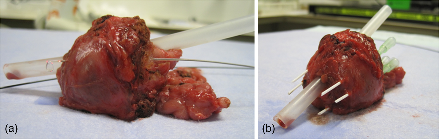 2.4.Correlation of 3-D OCT Data with Prostate HistopathologyFollowing OCT measurements, an independent pathologist diagnosed the histological slides according to our institute’s standard protocol. The prostate was placed in formalin over night for fixation with the IV catheters in place. On day 2, the pathologist colored the two prostate sides to indicate left and right and dissected the prostate into slices of 3 to 5 mm (lamellation). From these slices, a thin layer was skived for microscopic analysis. The contours of the OCT measurement trajectories, as well as areas of malignant tissue, were marked on the slides. All individual microscopic slides were reconstructed into a 3-D pathology representation showing the prostate contour, benign tissue, tumor, and OCT probe trajectories using AMIRA™. The 3-D OCT pullbacks and corresponding attenuation maps were manually coregistered, which allows for visual correlation of pathology and OCT data. Additionally, an overlay of quantitative attenuation plots and pathology was created. 3.ResultsThe calibration measurements in various Intralipid concentrations are depicted in Fig. 4, demonstrating a nonlinear increase of attenuation coefficient with increasing concentration. These values and nonlinear behavior, which is due to dependent and multiple scattering, are in concordance with our earlier published results.33,34 As shown in Fig. 5 and Table 1, the smallest difference in per probe is ; the largest difference in per probe is . The smallest difference in between probes is ; the largest difference in between probes is . For Intralipid concentrations within the scattering range of prostate tissue () two times the standard deviation of the measurements, an indication of the precision (reproducibility) of our measurement technique, was of the mean of the measured values. Table 1Mean optical attenuation coefficients per probe with range (visual representation in Figs. 1 and 2). Note that per probe the smallest and largest ranges in μoct are 0.06 and 0.33 mm−1, respectively. Between probes, the smallest and largest differences in measured μoct are 0.15 and 0.65 mm−1, respectively.
Fig. 4Attenuation measurements were validated by measurement of of samples with increasing concentrations of Intralipid®. The boxplots represent mean and range for all probes combined (see also Table 1). 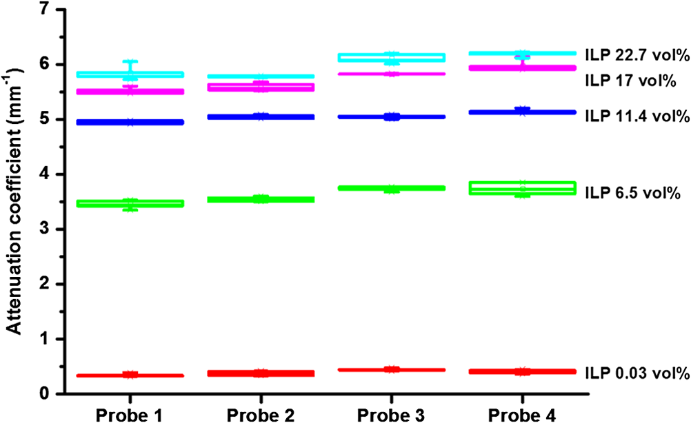 Fig. 5Interprobe variability was tested by measuring four probes five times in increasing concentrations of Intralipid. The boxplots represent the mean and range (see also Table 1). 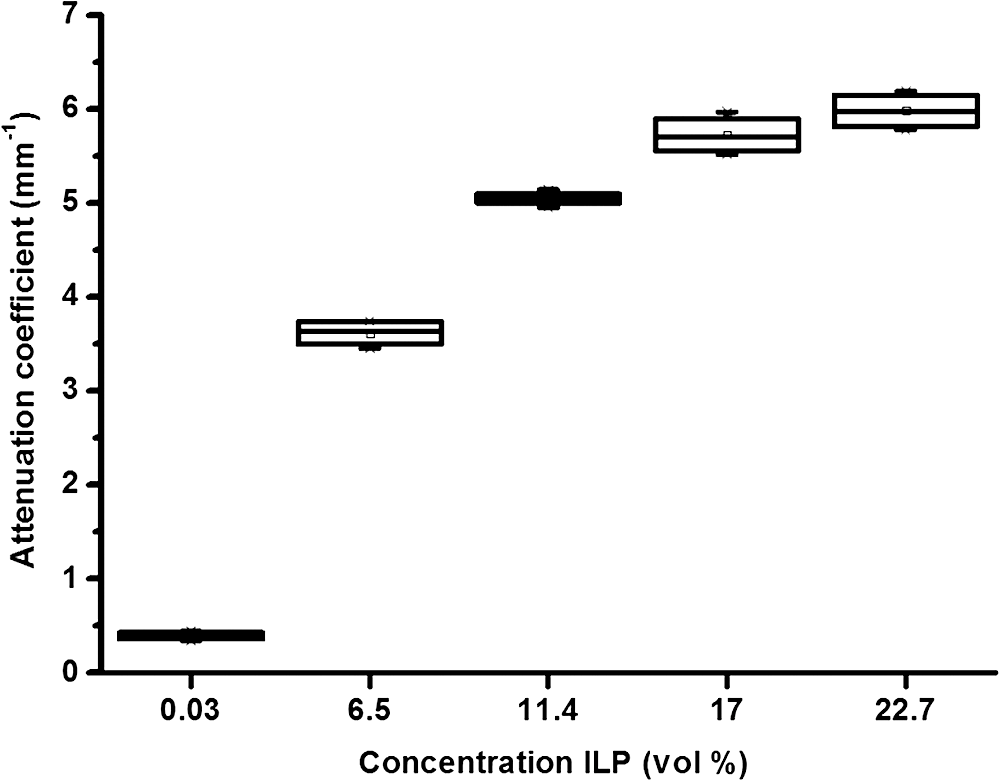 Analysis of the OCT data obtained in the prostate resulted in mean attenuation coefficients of for parts of the tissue that were classified as benign (SD: , minimum: , maximum: ) and for parts of tissue that were classified as malignant (SD: , minimum: , maximum: ). Figure 6(a) shows a 3-D representation of the OCT measurement with visualization of three separate B-scans. In Fig. 6(b), which was characterized as malignant tissue on pathology, glandular appearing structures can be observed. In Fig. 6(c), which was characterized as benign tissue on pathology, homogeneous prostate tissue can be seen. In Fig. 6(d), a cyst filled with clear fluid is shown, which the automated analysis recognizes as a high attenuation coefficient. The ring around the B-scans visually represents the attenuation coefficient (the same color scale is used as in Fig. 2). It is clear that the attenuation coefficient differs in prostate tissue. Fig. 6Structural properties of prostate tissue. (a) Three-dimensional (3-D) representation of an OCT measurement of prostate tissue with a visualization of three separate B-scans. (b) B-scan from malignant area (Gleason ) of the prostate. Glandular appearing structures are observed in these malignant areas (arrow). Optical attenuation coefficients in this area are high, indicated by the red ring around the raw data (visualizing the output of the automated attenuation analysis). (c) B-scan from a benign region of the prostate. In these benign areas, homogeneous tissue was seen, resulting in a low attenuation coefficient, indicated by the blue ring (visualizing the output of the automated attenuation analysis). (d) B-scan from an area in which a cyst was seen. In these irregular areas, attenuation coefficient matching is not always accurate, resulting in a high variation of attenuation coefficients, indicated by the multiple colors on the ring (visualizing the output of the automated attenuation analysis). The scale bar is 5 mm.  Figure 7 shows a prostate after histopathological evaluation. After fixation in formalin, the prostate was painted orange on the left side and blue on the right side. Subsequently, the prostate was sliced from base (slice 1) to apex (slice 8), and all slices were positioned with the same side up. The OCT measurement trajectories, indicated by the IV catheters, are very well visible. Four H&E stained microscopy slides per prostate slice were obtained and the pathologist indicated areas of tumor on these slides, as marked in red. These microscopic slides were overlaid on the overview picture of the prostate slices. Using AMIRA™, we reconstructed the prostate contour and lesion contours by stacking the slices in 3-D [Fig. 8(a)]. By plotting the St. Jude OCT measurements [Fig. 8(c)] and attenuation maps [Fig. 8(d)] in these reconstructed contours by using the holes of the IV catheters as a guide, we could estimate the distance between the slices (average slice thickness). Also, we were able to estimate which part of the OCT measurements went through tumor and which parts went through benign tissue. Finally, the information on coregistration was used to determine which B-scans corresponded to the sampled areas in the prostate slices. The attenuation information from these matched B-scans was also plotted in the picture of the prostate slices (Fig. 7, 1 to 8). Not all areas in which a high attenuation coefficient became apparent corresponded to areas of prostate cancer. Fig. 7Histopathological evaluation. The prostate was sliced from base (slice 1), to apex (slice 8), and all slices were positioned with the same side up. The pathologist indicated areas of tumor on the slides, as marked in red. The attenuation information from these matched B-scans were also plotted in the picture of the prostate slices (1 to 8). # corresponds to Fig. 6(b), * to Fig. 6(c), and ^ to Fig. 6(d). 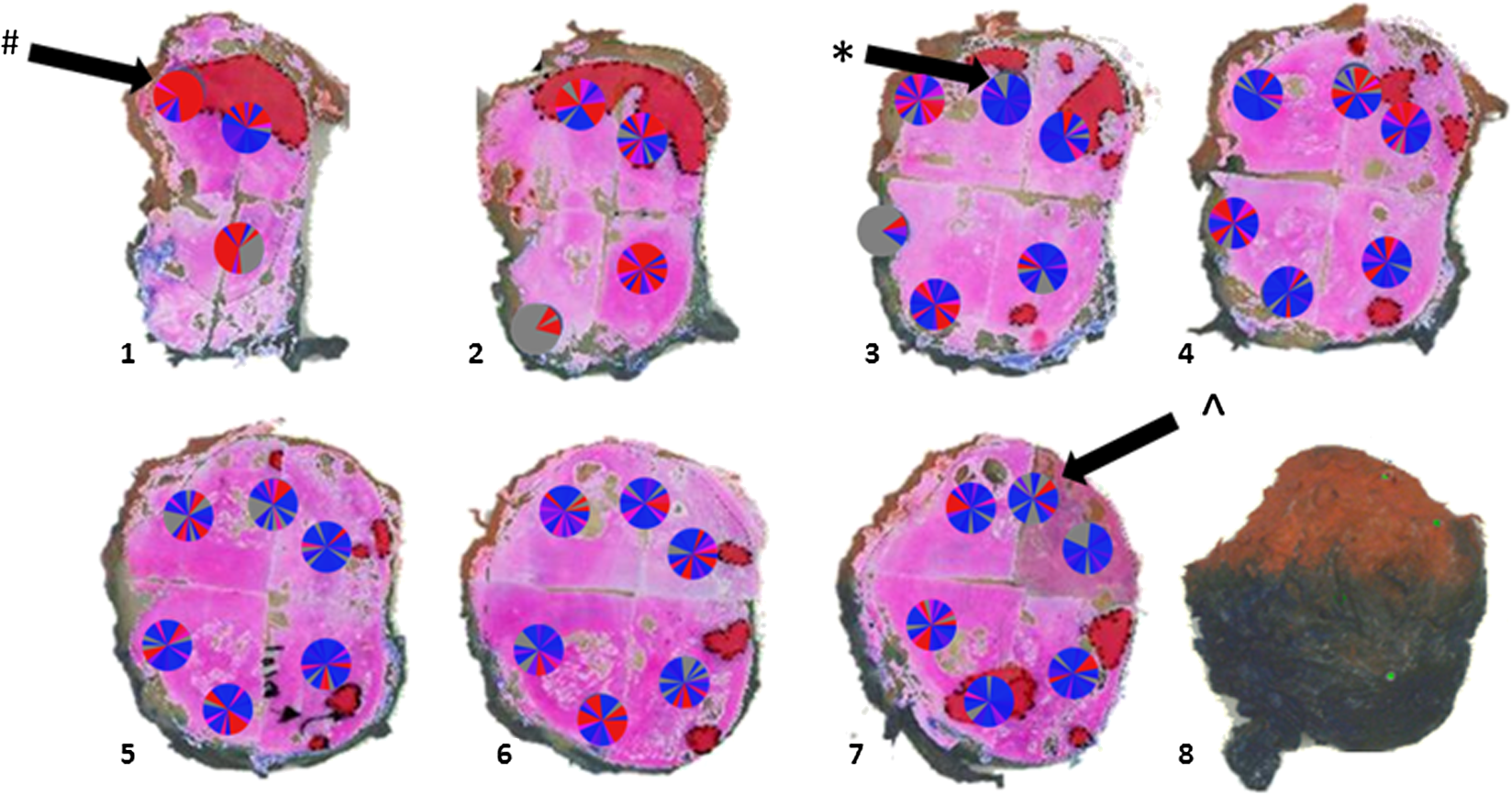 Fig. 83-D correlation to histopathology. (a) Using AMIRA™, we reconstructed the prostate contour (green) by stacking the slices from Fig. 6 in 3-D. (b) Because the pathologist outlined the tumor contours on the slides, we were able to reconstruct the tumors in 3-D. By plotting the (c) St. Jude OCT measurements and (d) attenuation maps in these reconstructed contours, based on the IV catheters that were visible in the slices, we could estimate which B-scans corresponded to the sampled areas in the prostate slices. The attenuation maps of these corresponding B-scans are overlaid in Fig. 7.  4.DiscussionWe demonstrate a method that allows for 3-D quantitative analysis of OCT optical attenuation coefficient datasets that may indicate a correlation with tissue disease status. This study is the first to show the feasibility of quantitative needle-based OCT in the prostate. This study is the first step toward real-time objective diagnosis of prostate cancer, a largely emphasized challenge in urology. Full clinical translation of OCT should build on three fundamental pillars. First, qualitative properties should be objectified with quantitative information, which can be spatial measurements from images (e.g., layer thicknesses), attenuation coefficients such as in our study, or more complex statistics related to tissue organization. A major challenge is relating measured optical properties to gold standard pathology diagnosis. This gap cannot be bridged without fundamental studies—far beyond the scope of our present contribution—that include both advanced OCT signal modeling and leveraging the potential of quantification of digital pathology. Second, the technology should be compatible with existing procedures and protocols. We presently use the clinically proven OCT equipment C7-XR™ OCT Intravascular Imaging System interfaced to a C7 Dragonfly™ Intravascular Imaging Probe (St. Jude Medical, St. Paul, Minnesota). Since the sterile probes are unpackaged just before measurements, prior calibration of the probes is not possible. We, therefore, devised an efficient, cost-effective procedure based on an easily obtained Intralipid™ suspension. Moreover, this study shows that intra- and interprobe variation is minimal, which suggests high data fidelity even if post hoc calibration is not possible (for example, because blood has entered the imaging catheter). However, the study shows that postmeasurement calibration of the probes improves measurement precision, since there is some small variation between the probes. Third, the future of prostate cancer will be image guided targeted diagnosis, likely by a combination of imaging technologies.39 Using TRUS, a location estimation of the OCT probe can be obtained. In addition to this, OCT visualizes the position of a lesion along the optical biopsy axis. It has been shown that when MRI data were fused with data from a conventional TRUS, the sensitivity increased drastically. More biopsies were found positive in the fused group and more malignant tissue was found per biopsy,40 even accomplishing results similar to transperineal 3-D prostate mapping biopsy.41 Our hypothesis is that integrating OCT in the combined results of MRI/TRUS fusion will further improve the diagnostic accuracy. Moreover, results will become objective and real time. For the diagnosis of kidney tumors, similar developments are ongoing. Projects are running to test the ability of OCT as a means of optical biopsy for kidney cancer (NCT02073110, Ref. 42) using the same OCT device as is used in our study. The few studies performed regarding OCT in the prostate focus on the qualitative interpretation of optical findings to identify surgical margins and neurovascular bundles.43–46 One manuscript described a difference between malignant and benign prostate tissue structures visualized with OCT; however, these results were not quantitatively analyzed.47 When the OCT technology further improves (smaller, higher-resolution, faster machines) and analysis software evolves (e.g., structure recognition, automatic learning, etc.), the technology will most likely become faster, more objective and more accurate. OCT is a new diagnostic modality in the prostate. We acknowledge the limitations that this study entails. First, the St. Jude system evaluates tissue every 0.1 mm, whereas whole mount pathology assesses the tissue in theory every 4 mm. Due to free hand slicing, this slice thickness varies in practice between 3 and 5 mm, creating OCT images uncertainty in the first slice. This matching-uncertainty is of non-negligible proportion, since every prostate slice has this variable slice thickness of 3 to 5 mm. Furthermore, we assumed in this study that the slice thickness is constant throughout the prostate slice. However, it is very well possible that a slice might be slightly wedge shaped in reality. Also, when a tumor is not present throughout the whole slice, it can cause matching issues (Fig. 9). All these aspects create uncertainty in the 3-D OCT histopathology matching and have to be overcome for further validation studies. Solving this issue is currently in progress by using a customized tool for dedicated pathology matching and slicing. Second, the St. Jude imaging probe does not have a marker that indicates angular probe position in tissue, so a method should be designed to register this. Further studies are in progress that provide larger numbers of patients and address the slicing and pathology-matching issues described above. Finally, in ex vivo measurements, blood flow and tissue perfusion are not present. In vivo measurements are needed to determine whether or not the results are reproducible. Fig. 9Schematic representation of histopathology matching challenges. Each blue block (numbered 1 to 8) represents a slice of prostate. The bold red lines on each left side of a blue block represent the pathology slide (part of the prostate that is actually visualized under the microscope). The striped bar in the middle represents an OCT scan, and each stripe represents a B-scan. The letters on the left side represent the possible scenarios. A, slice of prostate that looks benign but actually is half tumor (false negative); B, prostate slice that looks malignant and is malignant (true positive); C, prostate slice that looks malignant but is half benign (false positive); and D, prostate slice that looks negative and is negative (true negative). It is clear that because of the matching issues, the difference between benign and malignant attenuation coefficients becomes smaller.  5.ConclusionWe demonstrated the feasibility of needle-based 3-D quantitative 1300 nm OCT in prostate tissue as a first step toward objective and real-time digital diagnosis of prostate cancer. Fully automated attenuation coefficient analysis was performed over the full pullback. Optimal correlation with pathology was achieved by coregistration of 3-D OCT attenuation maps with 3-D pathology of the prostate. This approach may contribute to the current challenge of prostate imaging and the rising interest in focal therapy for reduction of side effects occurring with current therapies. However, in further research, the challenges of exact histopathology correlation as well as analysis of different cell types of the prostate need to be addressed. ReferencesR. Siegel, D. Naishadham and A. Jemal,
“Cancer statistics,”
J. Clin., 63
(1), 11
–30
(2013). http://dx.doi.org/10.3322/caac.21166 Google Scholar
F. Brimo et al.,
“Contemporary grading for prostate cancer: implications for patient care,”
Eur. Urol., 63
(5), 892
–901
(2013). http://dx.doi.org/10.1016/j.eururo.2012.10.015 EUURAV 0302-2838 Google Scholar
T. J. Wilt et al.,
“Radical prostatectomy versus observation for localized prostate cancer,”
N. Engl. J. Med., 367
(3), 203
–13
(2012). http://dx.doi.org/10.1056/NEJMoa1113162 NEJMAG 0028-4793 Google Scholar
A. Heidenreich et al.,
“EAU guidelines on prostate cancer. Part 1: screening, diagnosis, and local treatment with curative intent-update 2013,”
Eur. Urol., 65
(1), 124
–137
(2014). http://dx.doi.org/10.1016/j.eururo.2013.09.046 EUURAV 0302-2838 Google Scholar
H. U. Ahmed and M. Emberton,
“Active surveillance and radical therapy in prostate cancer: can focal therapy offer the middle way?,”
World J. Urol., 26
(5), 457
–467
(2008). http://dx.doi.org/10.1007/s00345-008-0317-5 Google Scholar
S. Rais-Bahrami et al.,
“Utility of multiparametric magnetic resonance imaging suspicion levels for detecting prostate cancer,”
J. Urol., 190
(5), 1721
–1727
(2013). http://dx.doi.org/10.1016/j.juro.2013.05.052 Google Scholar
W. E. Barzell and M. R. Melamed,
“Appropriate patient selection in the focal treatment of prostate cancer: the role of transperineal 3-dimensional pathologic mapping of the prostate—a 4-year experience,”
Urology, 70
(6 Suppl), S27
–35
(2007). http://dx.doi.org/10.1016/j.urology.2007.06.1126 Google Scholar
G. Onik and W. Barzell,
“Transperineal 3D mapping biopsy of the prostate: an essential tool in selecting patients for focal prostate cancer therapy,”
Urol. Oncol., 26
(5), 506
–510
(2008). http://dx.doi.org/10.1016/j.urolonc.2008.03.005 Google Scholar
M. M. Siddiqui et al.,
“Comparison of MR/ultrasound fusion-guided biopsy with ultrasound-guided biopsy for the diagnosis of prostate cancer,”
JAMA, 313
(4), 390
–397
(2015). http://dx.doi.org/10.1001/jama.2014.17942 JAMAAP 0098-7484 Google Scholar
A. M. Zysk et al.,
“Optical coherence tomography: a review of clinical development from bench to bedside,”
J. Biomed. Opt., 12
(5), 051403
(2007). http://dx.doi.org/10.1117/1.2793736 JBOPFO 1083-3668 Google Scholar
K. Barwari et al.,
“Differentiation between normal renal tissue and renal tumours using functional optical coherence tomography: a phase I in vivo human study,”
BJU Int., 110
(8b), E415
–E420
(2012). http://dx.doi.org/10.1111/j.1464-410X.2012.11197.x Google Scholar
M. T. Bus et al.,
“Volumetric in vivo visualization of upper urinary tract tumors using optical coherence tomography: a pilot study,”
J. Urol., 190
(6), 2236
–2242
(2013). http://dx.doi.org/10.1016/j.juro.2013.08.006 Google Scholar
E. C. Cauberg et al.,
“Quantitative measurement of attenuation coefficients of bladder biopsies using optical coherence tomography for grading urothelial carcinoma of the bladder,”
J. Biomed. Opt., 15
(6), 066013
(2010). http://dx.doi.org/10.1117/1.3512206 JBOPFO 1083-3668 Google Scholar
S. A. Faruqi, V. Arantes and M. S. Bhutani,
“Barrett’s esophagus: current and future role of endosonography and optical coherence tomography,”
Dis. Esophagus, 17
(2), 118
–123
(2004). http://dx.doi.org/10.1111/j.1442-2050.2004.00406.x Google Scholar
W. Kang et al.,
“Endoscopically guided spectral-domain OCT with double-balloon catheters,”
Opt. Express, 18
(16), 17364
–17372
(2010). http://dx.doi.org/10.1364/OE.18.017364 OPEXFF 1094-4087 Google Scholar
T. H. Tsai et al.,
“Structural markers observed with endoscopic 3-dimensional optical coherence tomography correlating with Barrett’s esophagus radiofrequency ablation treatment response (with videos),”
Gastrointest. Endosc., 76
(6), 1104
–1112
(2012). http://dx.doi.org/10.1016/j.gie.2012.05.024 Google Scholar
D. P. Poppas et al.,
“Nerve sparing ventral clitoroplasty preserves dorsal nerves in congenital adrenal hyperplasia,”
J. Urol., 178
(4 Pt 2), 1802
–1806
(2007). http://dx.doi.org/10.1016/j.juro.2007.03.186 Google Scholar
R. Wessels et al.,
“Optical coherence tomography in vulvar intraepithelial neoplasia,”
J. Biomed. Opt., 17
(11), 116022
(2012). http://dx.doi.org/10.1117/1.JBO.17.11.116022 JBOPFO 1083-3668 Google Scholar
M. A. Calin et al.,
“Optical techniques for the noninvasive diagnosis of skin cancer,”
J. Cancer Res. Clin. Oncol., 139
(7), 1083
–1104
(2013). http://dx.doi.org/10.1007/s00432-013-1423-3 JCROD7 1432-1335 Google Scholar
T. Gambichler, V. Jaedicke and S. Terras,
“Optical coherence tomography in dermatology: technical and clinical aspects,”
Arch. Dermatol. Res., 303
(7), 457
–473
(2011). http://dx.doi.org/10.1007/s00403-011-1152-x Google Scholar
E. Sattler, R. Kastle and J. Welzel,
“Optical coherence tomography in dermatology,”
J. Biomed. Opt., 18
(6), 061224
(2013). http://dx.doi.org/10.1117/1.JBO.18.6.061224 JBOPFO 1083-3668 Google Scholar
M. J. Grundeken et al.,
“Three-dimensional optical coherence tomography evaluation of a left main bifurcation lesion treated with ABSORB(R) bioresorbable vascular scaffold including fenestration and dilatation of the side branch,”
Int. J. Cardiol., 168
(3), e107
–108
(2013). http://dx.doi.org/10.1016/j.ijcard.2013.07.255 IJCDD5 0167-5273 Google Scholar
A. C. Papayannis et al.,
“Optical coherence tomography evaluation of drug-eluting stents: a systematic review,”
Catheter Cardiovasc. Interv., 81
(3), 481
–487
(2013). http://dx.doi.org/10.1002/ccd.24327 Google Scholar
M. Terashima, H. Kaneda and T. Suzuki,
“The role of optical coherence tomography in coronary intervention,”
Korean J. Intern. Med., 27
(1), 1
–12
(2012). http://dx.doi.org/10.3904/kjim.2012.27.1.1 Google Scholar
N. Bosschaart et al.,
“Optical properties of neonatal skin measured in vivo as a function of age and skin pigmentation,”
J. Biomed. Opt., 16
(9), 097003
(2011). http://dx.doi.org/10.1117/1.3622629 JBOPFO 1083-3668 Google Scholar
D. Faber et al.,
“Quantitative measurement of attenuation coefficients of weakly scattering media using optical coherence tomography,”
Opt Express, 12
(19), 4353
–4365
(2004). http://dx.doi.org/10.1364/OPEX.12.004353 Google Scholar
P. H. Tomlins et al.,
“Scattering attenuation microscopy of oral epithelial dysplasia,”
J. Biomed. Opt., 15
(6), 066003
(2010). http://dx.doi.org/10.1117/1.3505019 JBOPFO 1083-3668 Google Scholar
R. A. McLaughlin et al.,
“Mapping tissue optical attenuation to identify cancer using optical coherence tomography,”
Med. Image Comput. Comput. Assist. Interv., 5762 657
–664
(2009). http://dx.doi.org/10.1007/978-3-642-04271-3_80 Google Scholar
P. McCulloch,
“The IDEAL recommendations and urological innovation,”
World J. Urol., 29
(3), 331
–336
(2011). http://dx.doi.org/10.1007/s00345-011-0647-6 Google Scholar
P. McCulloch et al.,
“No surgical innovation without evaluation: the IDEAL recommendations,”
Lancet, 374
(9695), 1105
–1112
(2009). http://dx.doi.org/10.1016/S0140-6736(09)61116-8 LANCAO 0140-6736 Google Scholar
T. G. van Leeuwen, D. J. Faber and M. C. Aalders,
“Measurement of the axial point spread function in scattering media using single-mode fiber-based optical coherence tomography,”
IEEE J. Sel. Topics Quantum Electron., 9
(2), 227
–233
(2003). http://dx.doi.org/10.1109/JSTQE.2003.813299 IJSQEN 1077-260X Google Scholar
S. H. Yun et al.,
“High-speed optical frequency-domain imaging,”
Opt. Express, 11
(22), 2953
–2963
(2003). http://dx.doi.org/10.1364/OE.11.002953 OPEXFF 1094-4087 Google Scholar
J. Kalkman et al.,
“Multiple and dependent scattering effects in Doppler optical coherence tomography,”
Opt. Express, 18
(4), 3883
–3892
(2010). http://dx.doi.org/10.1364/OE.18.003883 OPEXFF 1094-4087 Google Scholar
V. M. Kodach et al.,
“Quantitative comparison of the OCT imaging depth at 1300 nm and 1600 nm,”
Biomed. Opt. Express, 1
(1), 176
–185
(2010). http://dx.doi.org/10.1364/BOE.1.000176 BOEICL 2156-7085 Google Scholar
D. M. de Bruin et al.,
“Optical phantoms of varying geometry based on thin building blocks with controlled optical properties,”
J. Biomed. Opt., 15
(2), 025001
(2010). http://dx.doi.org/10.1117/1.3369003 JBOPFO 1083-3668 Google Scholar
K. A. Vermeer et al.,
“Depth-resolved model-based reconstruction of attenuation coefficients in optical coherence tomography,”
Biomed. Opt. Express, 5
(1), 322
–337
(2013). http://dx.doi.org/10.1364/BOE.5.000322 BOEICL 2156-7085 Google Scholar
J. Schindelin et al.,
“Fiji: an open-source platform for biological-image analysis,”
Nat. Methods, 9
(7), 676
–682
(2012). http://dx.doi.org/10.1038/nmeth.2019 1548-7091 Google Scholar
A. Savitzky and M. J. E. Golay,
“Smoothing and differentiation of data by simplified least squares procedures,”
Anal. Chem., 36
(8), 1627
–1639
(1964). http://dx.doi.org/10.1021/ac60214a047 ANCHAM 0003-2700 Google Scholar
B. Turkbey, P. A. Pinto and P. L. Choyke,
“Imaging techniques for prostate cancer: implications for focal therapy,”
Nat. Rev. Urol., 6
(4), 191
–203
(2009). http://dx.doi.org/10.1038/nrurol.2009.27 Google Scholar
P. A. Pinto et al.,
“Magnetic resonance imaging/ultrasound fusion guided prostate biopsy improves cancer detection following transrectal ultrasound biopsy and correlates with multiparametric magnetic resonance imaging,”
J. Urol., 186
(4), 1281
–1285
(2011). http://dx.doi.org/10.1016/j.juro.2011.05.078 Google Scholar
J. P. Radtke et al.,
“Comparative analysis of transperineal template-saturation prostate biopsy versus MRI-targeted biopsy with MRI-US fusion-guidance,”
J. Urol., 193
(1), 87
–94
(2015). http://dx.doi.org/10.1016/j.juro.2014.07.098 Google Scholar
P. G. K. Wagstaff, P. Laguna Pes and J. J. M. C. H. de la Rosette,
“Optical biopsy to improve the diagnosis of kidney cancer,”
(2015) https://clinicaltrials.gov/ct2/show/NCT02073110?term=NCT02073110&rank=1 March ). 2015). Google Scholar
S. Chitchian et al.,
“Combined image-processing algorithms for improved optical coherence tomography of prostate nerves,”
J. Biomed. Opt., 15
(4), 046014
(2010). http://dx.doi.org/10.1117/1.3481144 JBOPFO 1083-3668 Google Scholar
S. Chitchian, T. P. Weldon and N. M. Fried,
“Segmentation of optical coherence tomography images for differentiation of the cavernous nerves from the prostate gland,”
J. Biomed. Opt., 14
(4), 044033
(2009). http://dx.doi.org/10.1117/1.3210767 JBOPFO 1083-3668 Google Scholar
P. P. Dangle et al.,
“The use of high resolution optical coherence tomography to evaluate robotic radical prostatectomy specimens,”
Int. Braz. J. Urol., 35
(3), 344
–353
(2009). http://dx.doi.org/10.1590/S1677-55382009000300011 Google Scholar
S. Rais-Bahrami et al.,
“Optical coherence tomography of cavernous nerves: a step toward real-time intraoperative imaging during nerve-sparing radical prostatectomy,”
Urology, 72
(1), 198
–204
(2008). http://dx.doi.org/10.1016/j.urology.2007.11.084 Google Scholar
A. V. D’Amico et al.,
“Optical coherence tomography as a method for identifying benign and malignant microscopic structures in the prostate gland,”
Urology, 55
(5), 783
–787
(2000). http://dx.doi.org/10.1016/S0090-4295(00)00475-1 Google Scholar
|
|||||||||||||||||||||||||||||||||||||||||


