Automatic correction of dental artifacts in PET/MRI

Claes N. Ladefoged; Flemming L. Andersen; Sune H. Keller; Thomas Beyer; Ian Law; Liselotte Højgaard; Sune Darkner; Francois Lauze

doi:10.1117/1.JMI.2.2.024009

9 June 2015 Automatic correction of dental artifacts in PET/MRI

Claes N. Ladefoged, Flemming L. Andersen, Sune H. Keller, Thomas Beyer, Ian Law, Liselotte Højgaard, Sune Darkner, Francois Lauze

Author Affiliations +

Journal of Medical Imaging, Vol. 2, Issue 2, 024009 (June 2015). https://doi.org/10.1117/1.JMI.2.2.024009

Abstract

A challenge when using current magnetic resonance (MR)-based attenuation correction in positron emission tomography/MR imaging (PET/MRI) is that the MRIs can have a signal void around the dental fillings that is segmented as artificial air-regions in the attenuation map. For artifacts connected to the background, we propose an extension to an existing active contour algorithm to delineate the outer contour using the nonattenuation corrected PET image and the original attenuation map. We propose a combination of two different methods for differentiating the artifacts within the body from the anatomical air-regions by first using a template of artifact regions, and second, representing the artifact regions with a combination of active shape models and k-nearest-neighbors. The accuracy of the combined method has been evaluated using 25 ¹⁸F-fluorodeoxyglucose PET/MR patients. Results showed that the approach was able to correct an average of 97±3% of the artifact areas.

1. Introduction

Combined PET/MR imaging systems have recently become available to clinical users.¹ The original MR-based attenuation map ( $μ$ -map) is obtained in a different manner depending on the vendor. The fully integrated PET/MR system (Biograph mMR, Siemens Healthcare)² uses the Dixon volumetric interpolated breath-hold examination sequence,³ from which a segmentation of the images is made into the four classes air, [linear attenuation coefficient (LAC) $μ = 0 {cm}^{- 1}$ ], lung ( $0.0224 {cm}^{- 1}$ ), fat ( $0.0854 {cm}^{- 1}$ ), and soft tissue ( $0.1 {cm}^{- 1}$ ). The accuracy of MR attenuation correction (AC) is challenged by susceptibility effects caused by dental fillings and metal braces.⁴^–⁷ The effect of a metal implant can be a signal void around the metal filling in the MR images [Figs. 1(a)–1(c)], resulting in the area incorrectly being set to air in the $μ$ -map [Fig. 1(d)].

Fig. 1

Illustration of two types of artifacts: (a)–(d) type A and (e)–(h) type B, the first breaching the anatomical volume, the second not: (a), (e) sagittal T1w MR image shown in transaxial orientation; (b), (f) fat, and (c), (g) water-image composition from in- and out-phase MR from Dixon VIBE sequence used for attenuation map segmentation; and (d), (h) MR-based attenuation map ( $μ$ -map) with dental artifact.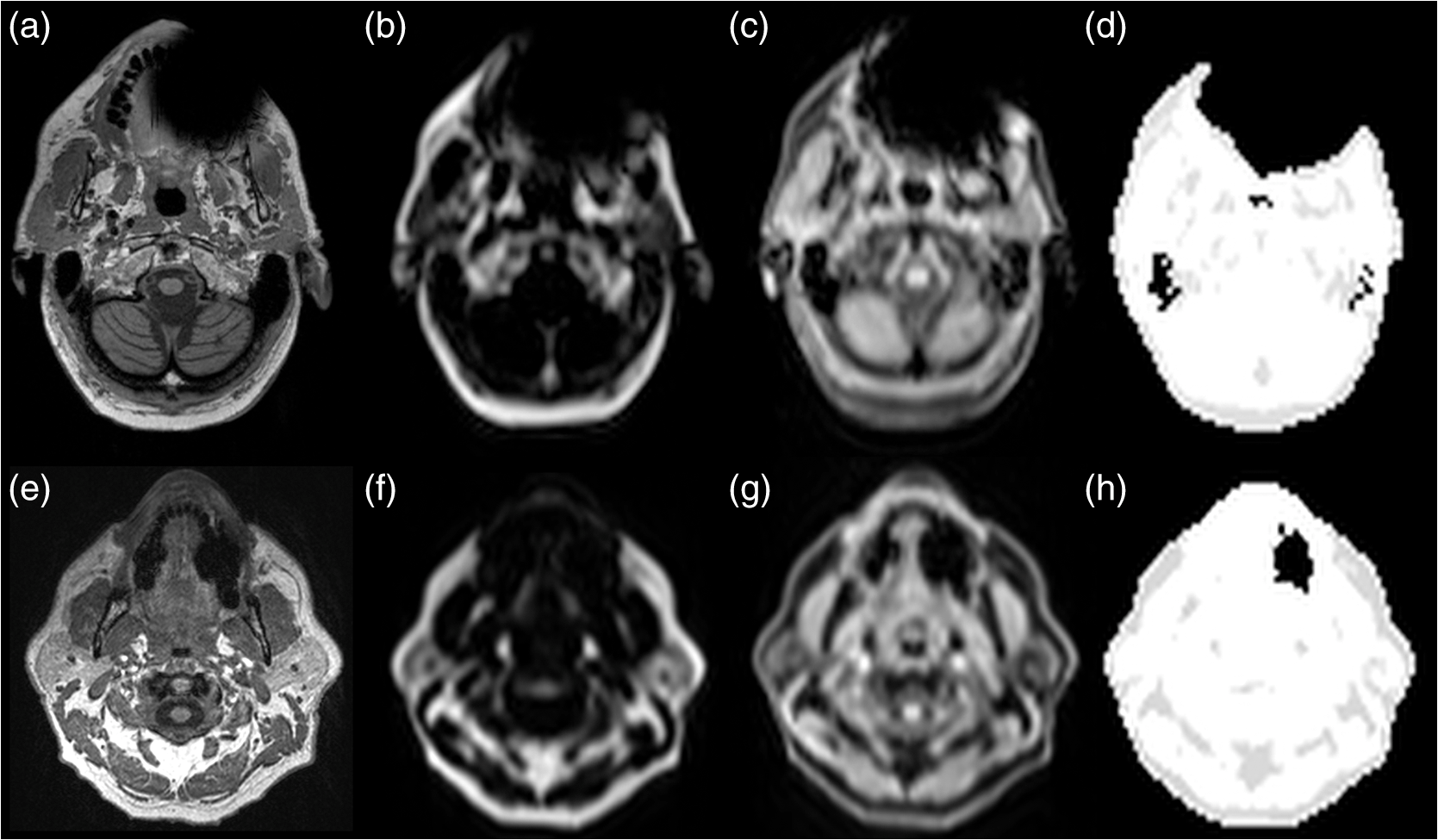

Prevailing techniques for calculating correct $μ$ -maps has been suggested in numerous literature cases. Methods based on the introduced time-of-flight technique are not discussed here, as it is not an option for current mMR. We refer to Ref. 8 for an extensive overview of the greatest number of the existing methods. None of these methods are focused on the task of correcting susceptibility artifacts in the dental region, which is currently without a satisfactory solution.⁹

The main challenge in all methods is corrupted data caused by metal implants. Several authors have investigated the use of PET images for outer contour delineation to compensate for truncation artifacts due to the limited MR field of view in whole-body imaging. The method proposed in Ref. 10 uses a maximum-a-posteriori algorithm to jointly estimate activity map and the missing parts of the corresponding attenuation map, whereas Ref. 11 locates the outer contour by looking for a PET signal in areas where truncation artifacts are expected. While being successful for truncation artifact correction, the performance of either method in the dental region has not been studied. The latter method depends on the existence of a significant PET signal in the voxels at the borders. This assumption is not always true regarding AC-PET images in the presence of larger artifacts. In most cases, however, a signal will be present, only significantly decreased. The decrease is not predictable, as it depends on the size and shape of the artifact.

Due to this fact, it is preferable to use the only image not influenced by susceptibility artifacts: the nonattenuation corrected (NAC)-PET image. An active contour algorithm is used in Ref. 12 to detect the contour on the NAC-PET images. This approach is similar to the approach we are presenting in this study; however, our study deviates by the segmentation algorithm and, more importantly, by the fact that we also handle the problem that the body contour segmented on the NAC-PET image is larger than the $μ$ -map. This problem is also noted by the authors of Ref. 12, who found the error had caused an overestimation of PET values of 6% and 8% in two lesions located in the neck region.

Correction of artifacts within the body was studied in Ref. 4. The authors proposed to use an atlas-based method in which artifact regions are outlined in 11 patients. The performance of the method has not been studied in patients with dental artifacts.

It has previously been shown that the artifact region can be much larger than the actual metal implant,⁶^,¹³^,¹⁴ and is usually oval shaped for round fillings.¹⁵ The size and shape of artifacts cannot be predicted just by knowing size, positioning, and material of an implant.¹⁶ An artificial connection to air-regions, such as the maxillary sinuses, can occur when the metal is located near these. Furthermore, if the implant is located near the anatomical surface, which is often the case with dental fillings, the artifact can appear connected to the background, as seen in Fig. 1(d). We chose to separate the artifacts into two types:

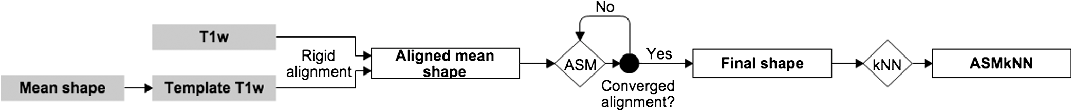
Type A: signal voids breaching the anatomical surface,
Type B: signal voids fully enclosed by soft tissue.

Both type A and B can be connected to the sinuses or other air regions.

We present a fully automatic method to correct for dental artifacts caused by metal fillings. For the contour delineation of type A artifacts, we extended the original segmentation method proposed by Chan and Vese¹⁷ with extra fitting terms evolving the contour, not only to match the PET image, but also in order to attract the contour toward the original $μ$ -map. Type B artifacts are handled by a combination of two methods. The first method fills signal voids overlapping a mask of the dental region defined on a MR-template generated on 30 patients. The second is a supervised learning-based method, employing active shape models (ASM)¹⁸ to locate a set of patient landmarks, followed by k-nearest-neighbors (kNN) to classify each of the signal voids by their offset on each of the landmarks, as in Ref. 19. For this work, we have employed realistically simulated artifacts in a patient cohort greater than the one used in Ref. 19. The artifacts are superimposed from four patients with dental artifacts following a coregistration. Having the original $μ$ -map without dental artifacts enabled us to directly quantify improvements obtained by the method. Finally, we combined all proposed methods into a final approach.

2. Materials

2.1.

Patients and Imaging Protocol

We selected 25 patients without dental artifacts (15 males, 10 females; median age: 60 y, range: 21 to 82 y). The patients were injected with a mean of 205 MBq ${}^{18}F$ -fluorodeoxyglucose (range: 191 to 337 MBq). The patients were all routine oncology or neurology patients in the context of a clinical study approved by the local ethical committee. All patients gave their written informed consent for the PET/MR examination. They were positioned head first, with their arms down, on the fully integrated PET/MR system (Biograph mMR; VB18p, Siemens Healthcare²), and data was acquired over a single bed position of 25.8 cm covering the head and neck. The emission acquisition time was 10 min. The PET images used in this study were reconstructed with and without MR-AC using three-dimensional (3-D) ordinary Poisson-ordered subset expectation maximization (4 iterations, 21 subsets, 3 mm Gaussian filter postreconstruction) on $344 \times 344 \times 127$ matrices ( $0.8 \times 0.8 \times 2.0 {mm}^{3}$ voxels) into the resulting images. The DIXON-water images and $μ$ -maps were reconstructed on $192 \times 126 \times 128$ matrices ( $2.6 \times 2.6 \times 3.1 {mm}^{3}$ voxels). The sagittal T1-weighted (T1w) MPRAGE images, used in the correction algorithm, had a matrix size of $512 \times 512 \times 192$ ( $0.5 \times 0.5 \times 1 {mm}^{3}$ voxels).

2.2.

Construction of Artifact $μ$ -maps

We created four artifact masks by manually segmenting four common types of dental artifacts on real patient data (Fig. 2). Artifact 1 and 2 are artifacts of type A, and artifact 3 and 4 are type B. Artifact 1 [Fig. 2(a)] is a large artifact that removes most of the mandibular and nose regions. The artifact exceeds the anatomical surface and is always connected artificially to the sinuses. Artifact 2 [Fig. 2(b)] is bilateral and connected both to the background and often also to the sinuses. Artifact 3 [Fig. 2(c)] is a unilateral artifact in the inferior left part of the mouth, which is never connected to anatomical air-regions. Artifact 4 [Fig. 2(d)] is also a unilateral artifact, but compared to artifact 3 is more than twice its size, and located in the superior left part of the mouth, meaning it is often connected to the left maxillary sinus.

Fig. 2

Patient data of the four real artifacts used to create the simulated are masked in red as seen on the sagittal and transaxial orientations [(a) and (b): type A, (c) and (d): type B]. (a) Large artifact removing the nose and mouth regions; (b) bilateral artifact connected to the background and sinuses; (c) unilateral in inferior part of the mouth, and (d) unilateral in superior part of the mouth.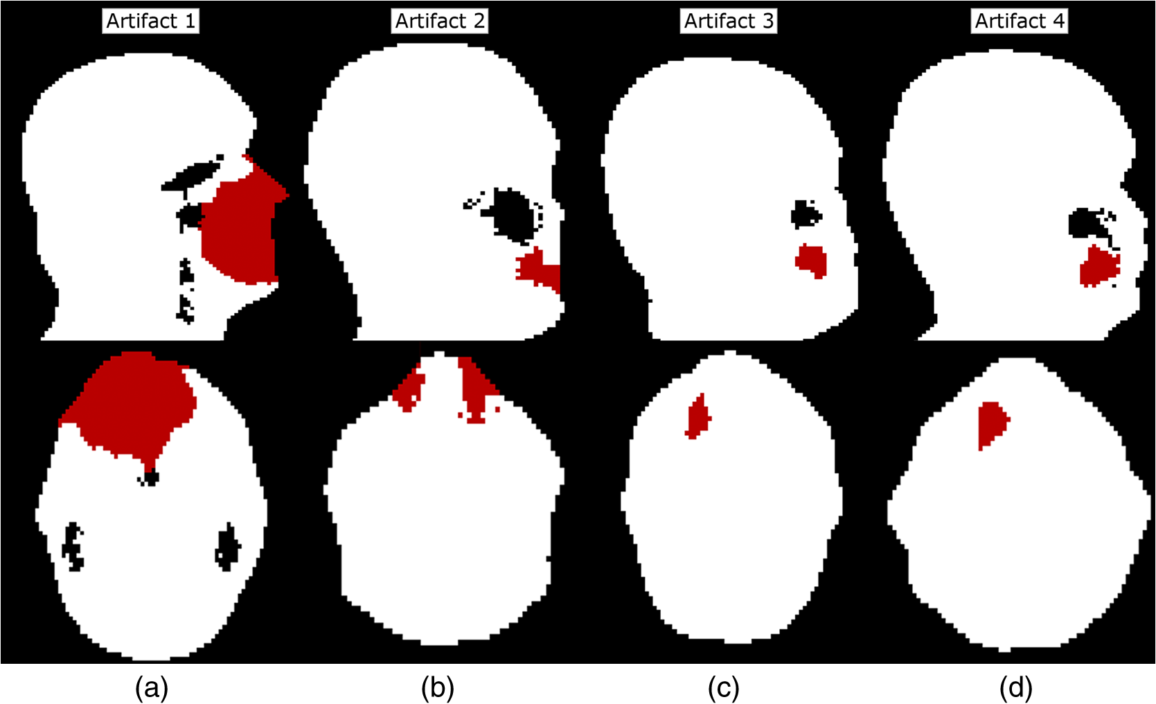

The artifacts were applied to 25 patient artifact free $μ$ -maps using semiautomatic alignment of the simultaneously acquired AC-PET, T1w and DIXON-water images to the patients with true artifacts using minctracc (McConnell Imaging Center, Montreal²⁰). The objection function of the Procrustes alignment was cross-correlation. By substituting soft tissue voxels with values representing air in the masked area we created $4 \times 25$ $μ$ -maps with dental artifacts and corresponding ground truth $μ$ -maps. The placement of the simulated artifacts were visually inspected to ensure that the listed specific properties were maintained for all subjects within each artifact type.

3. Methods

In the following, we present how to handle type A artifacts; that is signal voids breaching the anatomical surface, and type B artifacts; that is a separation from anatomical signal voids within the body.

3.1.

Type A Artifact Correction

Applying an active contour algorithm to the NAC-PET image [e.g., Fig. 3(a)] removes the connection of the artifact void to the background. However, the boundary on the NAC-PET volume is different than the original $μ$ -map, as the volume with PET uptake tends to be larger than the segmentation of the anatomical volume, as it was also reported in Ref. 12, and shown in Fig. 3(b). To address this problem, we present a slice-by-slice-based method. The full method consists of following steps:

Chan–Vese segmentation
Boundary estimation from the NAC-PET image using the original Chan–Vese (CV) active contour algorithm.
First erosion of segmented image
A postprocessing refining the segmentation where the $μ$ -map is known.
Postsegmentation
A segmentation that incorporates both the NAC-PET image as well as the original $μ$ -map.
Second erosion of segmented image
A postprocessing refining the new segmentation where the $μ$ -map is known.
The first segmentation and erosion were performed to obtain a coarse estimate of the PET volume. This volume was compared to the $μ$ -map in order to detect and estimate the size of any dental artifacts. By relating the estimated artifact sizes to fitting term weights, we performed a second segmentation and erosion step where the $μ$ -map was incorporated. We now proceed to a more thorough description of these steps.

Fig. 3

(a) Nonattenuation-corrected PET image and (b) segmented outer area (blue) of (a) and binary $μ$ -map mask (red) overlaid into (a). Notice the outer contour of the nonattenuation corrected (NAC)-PET image is different from that of the $μ$ -map. The grid illustrates the posterior and anterior half of the volume, and the three yellow points are the points used in the erosion of that slice.

3.1.1.

Chan–Vese segmentation

The CV algorithm¹⁷ segments an image $u_{0}$ by dividing it into two segments whose average values differ the most, while maintaining contour regularity. Segmentation is obtained by minimization of the following function

Eq. (1)

E_{CV} (ϕ, c_{i}, c_{o}) = μ \int | \nabla H (ϕ) | + ν \int H (ϕ) + λ_{i} \int_{Ω} H (ϕ) {| u_{0} - c_{i} |}^{2} + λ_{o} \int_{Ω} H (- ϕ) {| u_{0} - c_{o} |}^{2},

where

ϕ

is the level set function used to delineate two regions, the inner region corresponding to

ϕ \geq 0

and the outer one corresponding to

ϕ < 0

, while

c_{i}

and

c_{o}

are easily shown to be an average image values for the inner and outer regions, respectively. Here, the two regions separated are the patient and background, and the inner region refers to the patient volume. The function

H (t)

is the Heaviside function,

H (t) = 1

if

t \geq 0

, and

H (t) = 0

otherwise. The first term of Eq. (1) controls the length of the region boundary, while the second controls the volume of the inner region. In this work we have ignored it, setting

ν = 0

. Following,¹⁷ we used a regularized version of

H

. The solution was obtained by gradient descent as in Ref. 17.

For the purpose of estimating model parameters, we first segmented the NAC-PET volume using Eq. (1) where we initialized the contour at the position of the $μ$ -map and set the parameters $λ_{i} = λ_{o} = 100$ and $μ = 1$ . The high value for the $λ$ terms was selected to ensure that the contour placed itself on the outside of the NAC-PET volume.

3.1.2.

First erosion of segmented image

The CV segmented volume is larger than the original $μ$ -map. Assuming that the artifact does not extend to the posterior half of the $μ$ -map [see the black box in Fig. 3(b)], we have minimized the overestimation by doing the following for each slice:

1. Perform an erosion on the segmented image with a disk size equal to the maximum distance between the found contour and the original $μ$ -map at the three extreme points located posterior, left and right on the transaxial segmented image [Fig. 3(b)].
2. Insert $μ$ -values if the erosion removed valid $μ$ -map values.
3. Overwrite the lower half of the segmented volume with the original $μ$ -map.

For each slice, the posterior half was determined by locating the two most extreme points in the lateral direction, and splitting the volume in two [Fig. 3(b)].

3.1.3.

Postsegmentation

To force the contour toward the true anatomical boundary, we extended the original segmentation method in Eq. (1) by two extra fitting terms to match the original $μ$ -map. The first fitting term attracts the contour towards the $μ$ -map. The second fitting term prevents the contour from evolving into the $μ$ -map. The resulting level set segmentation functional is defined by

Eq. (2)

E (ϕ) = E_{CV} (ϕ) + \frac{λ_{{MR}_{i}}}{2} \int_{Ω} {[H (ϕ) - χ_{MR}]}^{2} + \frac{λ_{{MR}_{o}}}{2} \int_{Ω} {[H (- ϕ) - (1 - χ_{MR})]}^{2},

where

E_{CV} (ϕ)

is Eq. (1) and

χ_{MR}

is the binary map, which is 1 where the original

μ

-map differs from zero. The parameter

λ_{{MR}_{i}}

controls the similarity of the new level curve and the original

μ

-map contour. The level set function

ϕ

was initialized at the position of the original

μ

-map. In contrast to the presegmentation step, the set of parameters

(μ, λ_{o}, λ_{i}, λ_{MR}, λ_{{MR}_{i}}, λ_{{MR}_{o}})

as well as the gradient descent parameters, the artificial time step in the gradient descent, denoted

τ

, and the number of iterations,

i

, were tabulated using the estimated artifact size (Table 1). The area parameter

ν

was still set to 0. The estimated size of the artifact was obtained by subtracting the original

μ

-map from the presegmentation, followed by a smoothing and thresholding of it (Fig. 4). Table 1 was created empirically by testing a large set of parameter combinations and validating them on real patients with dental artifacts.²¹

Table 1

Lookup table to convert size of artifact to parameters.

Pixels	μ	λo	λi	λMRi	λMRi	τ	i
$> 500$	10	100	20	1	1	50	100
$> 450$	10	70	20	1	1	50	100
$> 400$	10	60	20	1	1	50	100
$> 350$	5	50	20	1	1	30	75
$> 300$	5	40	20	1	1	30	75
$> 250$	5	30	15	1	1	30	75
$> 200$	5	20	15	1	1	30	75
$> 100$	5	10	10	1	1	30	75
$> 0$	3	7	7	1	1	15	50
$= 0$	1	5	5	0.1	1	10	30

Fig. 4

Steps to compute size of an artifact in a slice: (a) NAC-PET image, (b) segmented and eroded image found from (a), (c) original $μ$ -map mask, (d) difference image between (b) and (c), and (e) smoothed and thresholded version of (d) shown in red on $μ$ -map from (c) in white.

It has previously been reported¹⁵ that metal implant induced artifacts are usually ball-shaped or elongated, which leads to following assumptions exemplified in Algorithm 1.

• Artifact size does not vary dramatically between neighboring slices. Perform a local smoothing.
• An artifact always spans several consecutive slices. Remove outliers.
• Artifact size decreases away from the slice(s) where they peak. If an artifact is found, the artifact size can be propagated to neighboring slices ensuring that all slices containing the artifact are corrected.

Algorithm 1

Regularizing the list of artifact sizes. The variable p represents the array of found artifact pixels for each of the slices. The regularized list of affected pixels for each slice is denoted pnew.

1: for $i = 0$ to ( $length (p)$ ) do

2: if $p (i - 1) > p (i)$ and $p (i + 1) > p (i)$ then

3: % If the current slice has a smaller artifact than both of its neighbors, we update the artifact size to the lowest of the neighbors

4:

p_{new} (i) \leftarrow \min (p (i - 1), p (i + 1))

5: end if

6: if $p (i) > 0$ and $sum (p (i - 2), p (i - 1), p (i + 1), p (i + 2)) = = 0$ then

7: % If the slice has an artifact, but none of its neighbors found any, we consider it an outlier

8:

p_{new} (i) \leftarrow 0

9: else if $p (i) > 0$ then

10: % If several slices found artifact pixels, we assume the neighboring slices are also affected. The size of the window w is determined by the number of artifact pixels in the current slice

11:

w \leftarrow floor (p (i) / 50)

12: % Find the maximum number of artifact pixels

13:

\max^{w} \leftarrow \max (p (i - w : i + w))

14: % Update all neighboring slices within the window

15:

p_{new} (i - w : i + w) \leftarrow \max^{w}

16: end if

17: end for

This regularization is done prior to the postsegmentation step.

3.1.4.

Second erosion of segmented image

We increased the parameters $λ_{i}$ and $λ_{o}$ , controlling the similarity of the new level curve and the original $μ$ -map contour, in the slices with large artifacts. Unfortunately, this causes the contour to diverge towards the result of the nonextended CV. To counter this effect, we performed the same erosion and overwriting of image data as in the second step of this method (Sec. 3.1.2). Finally, identified artifact regions in the $μ$ -map were filled with a value representing soft tissue ( $0.1 {cm}^{- 1}$ ). The resulting $μ$ -map is denoted eCV, shorthand for extended CV.

The flowchart of the eCV method is illustrated in Fig. 5.

Fig. 5

Flowchart of the extended Chan–Vese method.

3.2.

Type B Artifact Correction

The following presents a combination of two methodologies in handling type B artifacts, i.e., the separation of signal voids caused by artifacts from anatomical signal voids. Common for both of these is that they attempt to locate and separate the dental area, where only artifact signal voids can be present, from the rest of the head.

3.2.1.

Template with mask

To locate the dental area, we introduced external knowledge in the form of a template with the area of potential dental artifacts. The MR water image of 30 patients without dental artifacts were aligned, and an average image was computed and used as template. The alignment to the first patient was done by maximizing a cross-correlation–based objective function using a 12 parameters affine alignment procedure (minctracc, McConnell Imaging Center, Montreal²⁰). We applied the same transformation to the $μ$ -maps, in order to create a probability map of allowed air regions [Fig. 6(a)]. Having a map of the area where signal voids are allowed to be, we subsequently created a mask of the dental area where any signal void is considered an artifact [Fig. 6(b)]. For a new patient, we first aligned the water image to the template, applying the same transformation to the $μ$ -map. We filled the signal voids in the patient that overlapped with the dental area mask with a value representing soft tissue. The resulting $μ$ -map is denoted Template.

Fig. 6

(a) Water-template with mask of air-regions from 30 patients without dental artifacts and (b) water-template with mask of dental region outside the air-regions.

3.2.2.

Active shape models

In addition to the method of identifying the dental area by alignment to a template, we here attempt to identify the location of each voxel by their position relative to the anatomical surroundings. The surroundings will here be a set of predefined anatomical landmarks. We chose nine landmarks in the midsagittal slice of the T1w MR image, six of which were located at a border with high intensity in the image, and three within the brain. An example of the chosen slice of a T1w image is shown in Fig. 7(a), with the nine landmarks overlaid.

Fig. 7

(a) Landmarks on T1w; (b) search for displacement patch in local neighborhood around the landmark under the nose, where the red point depicts the current landmark placement and green depicts the best match; (c) first step in next iteration where the grid has been moved and width between points decreased; (d) sample points in the dental artifact region (red) and in the nonartifact region (green); and (e) scatter plots of offset between the sample points and two of the landmarks.

In short, the proposed method consists of a point distribution model (PDM) that contains parameters of the mean, covariance, eigenvalues, and eigenvectors of a training set of shapes manually drawn on a set of patients. An ASM then automatically places the landmarks in the T1w image of a new patient, using the PDM, as well as local appearance information around each point. We identified the artifacts in the dental region by their offset to the anatomical landmarks using a simple kNN search. The feature space was built by manually sampling air voxels in the patients from the training set used to construct the PDM. The flowchart of the method, denoted ASMkNN, is illustrated in Fig. 8. We will now proceed to a more thorough description of these steps.

Fig. 8

Flowchart of the ASMkNN method.

In order to build the PDM, we followed Cootes and Taylor:¹⁸ first, we used a full functional generalized Procrustes analysis (translation, rotation, and scaling) to align the training shapes, drawn on seven patients without artifacts, to a mean shape and computed the PDM parameters via principal component analysis. After alignment, we computed a patch average $r_{i}$ from patches centered around the original locations in each of the training shapes at each point ${\bar{x}}_{i}$ of the mean shape. In a similar manner to to Ref. 18, we limited the weight vector, ensuring that the new shape conforms with the shape model, to ensure that the new shape is similar to the training shapes.

To initially place the mean shape on a new patient T1w MR image, we computed a rigid registration from the T1w image of a patient in the training group to the new T1w image, and applied the same transformation to the shape from the training set image.

We optimized on local appearance: for each point in our shape we iteratively found the displacement that best aligned the precomputed average patch to the actual image content patch at a corresponding point, by searching in a local grid centered at the point. We projected the displacement so as to produce a shape conforming to the shape model as in Ref. 18. In Figs. 7(b) and 7(c) we show two iterations of the algorithm. We increased local resolution at each iteration by reducing the width between grid points. This procedure was applied to model both global and local shape movements.

3.2.3.

k-nearest neighbors

Each pixel $(p_{x}, p_{y})$ in a signal void was represented by its offset to each of the nine landmarks. Thus, each pixel in a signal void was represented by a vector of nine features, each defined as

Eq. (3)

v_{i} = (x_{i} - p_{x}, y_{i} - p_{y}),

where

(x_{i}, y_{i})

are the coordinates of landmark

i

. For five patients in the training set, we manually labeled 650 pixels belonging to air-regions in all areas of the head (labeled

+ 1

), and 210 pixels belonging to artifacts (labeled

- 1

) [Figs. 7(d) and 7(e)].

We trained our kNN for the optimal number $K$ of neighbors using five-fold cross validation on our 860-feature vectors for each landmark, and found that $K = 5$ gives the best separation of classes.

Using kNN on the full set of feature vectors, we classified pixels for the nine landmarks individually for each new patient, and employed a majority vote on the result

result = {\begin{cases} Air & if \sum_{i = 1}^{9} kNN (v_{i}) > 0 \\ Artifact & otherwise, \end{cases}

where

kNN (v_{i})

finds the label for a pixel in respect to the landmark

(x_{i}, y_{i})

using the distribution of offsets in the training set. The resulting

μ

-map was denoted ASMkNN.

3.3.

Combining Correction Methods

3.3.1.

Postprocessing on partly filled signal voids

Following constraints were applied to handle artificial signal voids connected to anatomical signal voids. Voids filled more than a predefined threshold (80%) were considered artifact voids, and were thus filled to 100%. Voids filled less than 10% were considered as errors if the size of the filled area was less than 0.5 mL. We applied this to all $μ$ -maps and denoted the resulting $μ$ -maps with a _pp suffix.

We combined the two methods ASMkNN and Template by applying a simple OR and an AND operation of the corrected areas found by the two methods. The results were denoted ASMkNN_pp_(or/and)_Template_pp. For type A artifacts we used the output of eCV as input to the correction methods ASMkNN and Template. This resulted in the $μ$ -maps eCV_ASMkNN and eCV_Template.

3.3.2.

Reinsertion of actual air-regions

Due to possible artifacts created by eCV we wished to reinsert the feasible air-regions. From the template-based correction method we had a map of possible air-regions from 30 patients without dental artifacts [Fig. 6(a)]. To account for patient variability, we computed a binary mask of air-regions by setting a voxel to air if at least one-third of the training data indicated air. By aligning this map to the $μ$ -maps, we obtained an estimate of possible air-regions. We reinserted air in the voxels filled by eCV that overlapped with the mask. Figure 9 illustrates this for a patient with artifact 1. The artifact $μ$ -map is shown in (b), and the resulting $μ$ -map after eCV is shown in (c). By comparing to the original shown in (a), it is clear that the artifact is connected to the patient’s right sinus, and the correction method has therefore filled parts of it. The mask of likely air-regions reinserts air in filled regions that it overlaps with, as shown in (d). The new $μ$ -maps are denoted eCV_ASMkNN_air and eCV_Template_air.

Fig. 9

Effect of the air correction algorithm: (a) ground truth $μ$ -map, (b) $μ$ -map with Artifact 1 inserted. Notice the artifact has connected the background to the left maxillary sinus in the image. (c) Result of eCV where the artifact has been filled, including a large part of the sinus, and (d) result of eCV_ASMkNN_air which has reinserted an estimation of the sinus.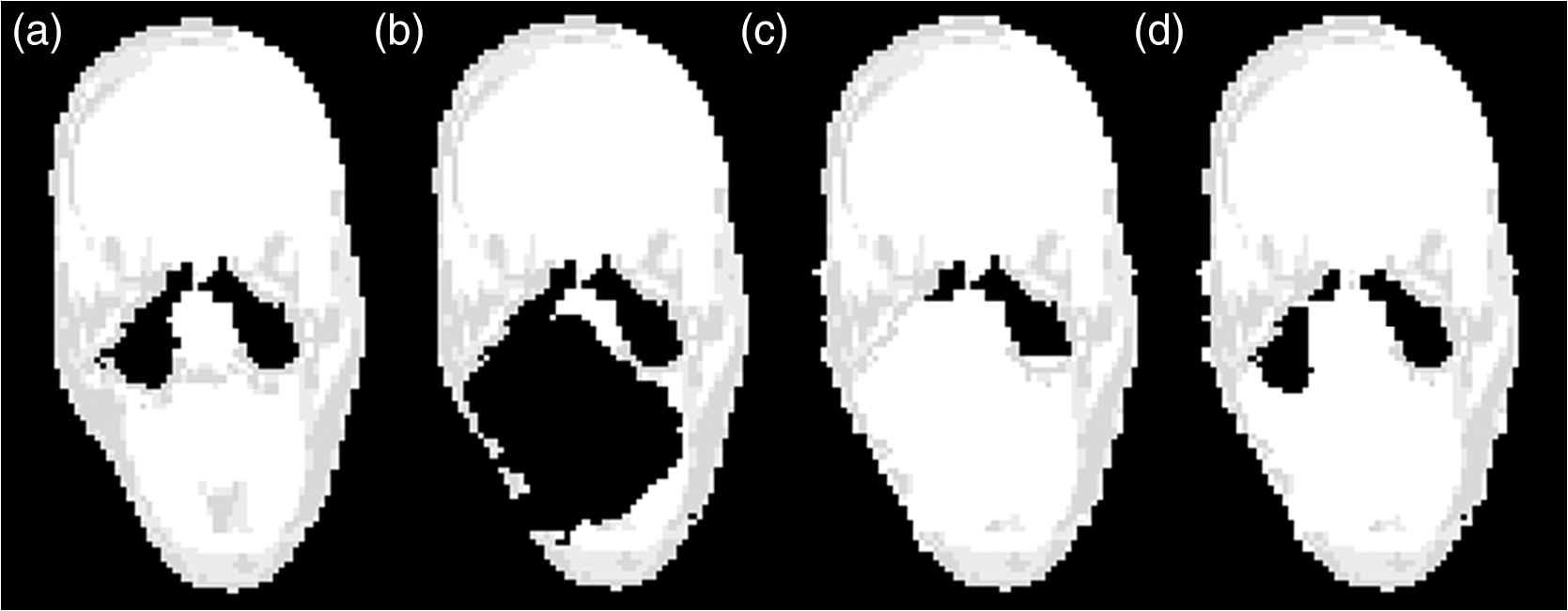

A flowchart of the combination of all the methods and their interplay is illustrated in Fig. 10.

Fig. 10

Flowchart of methods. From left: the four input image types used in the methods, the type A correction step, the type B correction steps. The latter is composed of four separate steps used in a feed-forward sequence. Each of the methods is evaluated separately.

3.4.

Quality Measures

As in Ref. 22, we assume that improved $μ$ -maps lead to better PET image quality. Therefore, our method was applied to patients with simulated artifacts, and evaluated by measuring the deviations from the ground truth $μ$ -maps without the artifacts. For each of the corrected $μ$ -maps (Fig. 10), we computed the $precision = tp / (tp + fp)$ , $recall = tp / (tp + fn)$ , and their harmonic mean $F_{1} = 2 \cdot precision \times recall / (precision + recall)$ , used to test the accuracy, where tp, fp, and fn are the number of true positive, false positive, and false negative voxels identified using the ground truth and the segmented $μ$ -maps.

4. Results

4.1.

Type A Artifacts

We now present the results for each of the four artifacts; see Fig. 2 for reference.

4.1.1.

Artifact 1 [Fig. 2(a)]

Figure 11 illustrates the results for a patient with artifact 1, where (a) shows a volume rendering illustrating the surface recovery, as well as the overestimated areas, such as the nose. Figure 2(b) shows the attenuation maps used to reconstruct the PET images in (c). Notice the similarity of the left and right image in each, compared to the middle image. A relative difference plot of the PET images reconstructed with the original $μ$ -map without artifacts versus artifact 1 and the eCV_ASMkNN_air_pp $μ$ -map, respectively, is shown in Fig. 11(d). Notice the substantial differences in the left image inside as well as outside the dental region. These differences have been corrected by the proposed approach. The only remaining differences are relatively insignificant ( $< 10 %$ ) at the bottom of the chin and at the edge of air regions within the mouth caused by local overestimation of the contour. This overestimation can be observed when comparing the left and right volume-rendered surfaces in Fig. 11(a).

Fig. 11

Effect of artifact 1 and the correction method. Relative difference images only showed for voxels with SUV $> 0.5$ in the original AC-PET: (a)–(c) the original $μ$ -map, (d), (e) the simulated artifact 1, and (f), (g) the corrected one using eCV_ASMkNN_air_pp.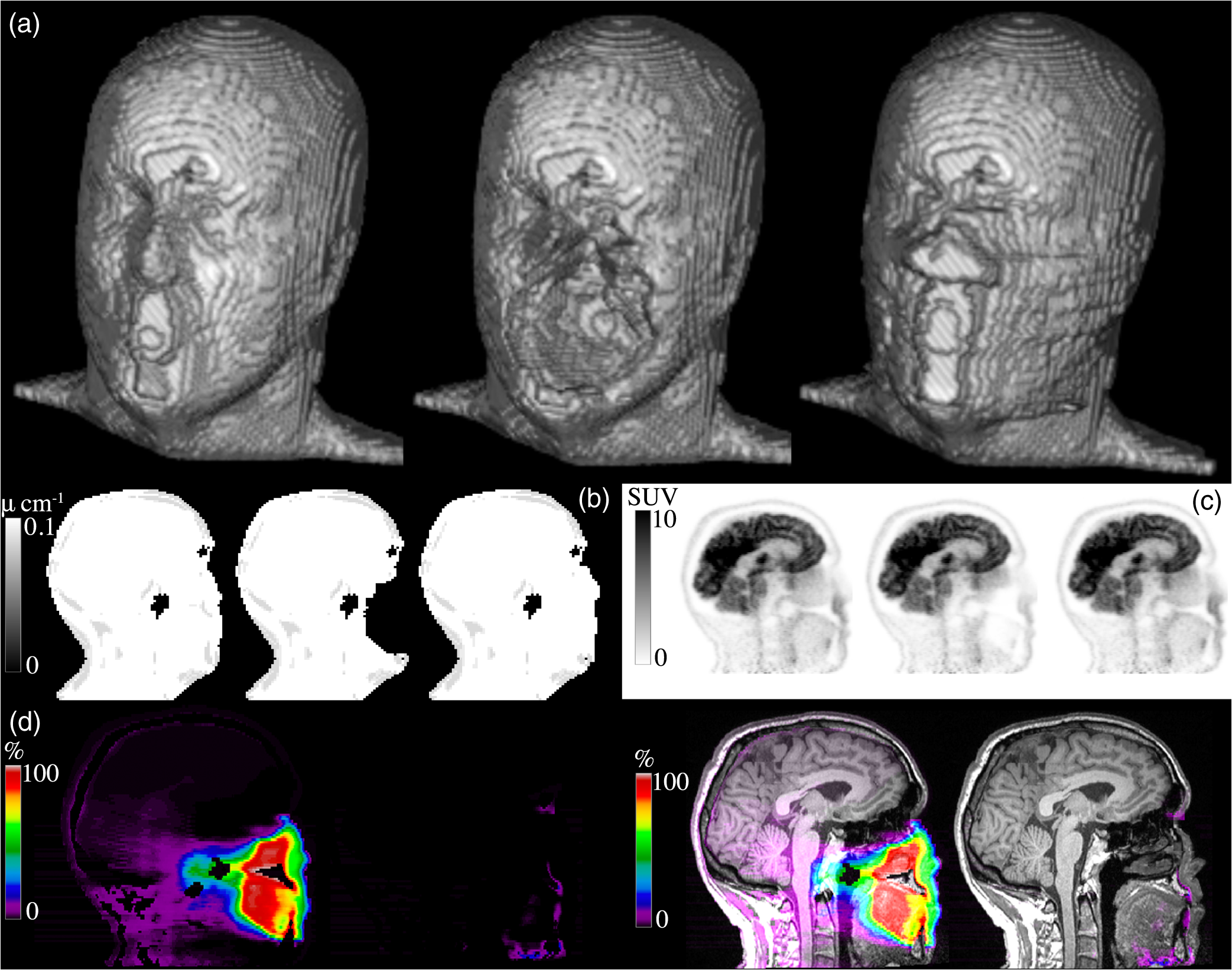

The best correction method for artifact 1 was eCV_ASMkNN_air_pp (Table 2). By using this method we filled 96% of the artifact volumes with a precision of 0.74, where 1 indicated no false positives and 0 indicated only false positives. Parts of the sinuses as well as voxels outside the volume and around the nose were incorrectly filled. Comparing eCV and eCV_ASMkNN_air_pp with the original $μ$ -map, we could measure to which degree the air-regions are recovered in the correction method. The average volume of the air-regions across all patients was 36 mL. Using eCV we filled an average of 9.5 mL in the air-regions, which was limited to 5.3 mL when using eCV_ASMkNN_air_pp.

Table 2

Precision (P), Recall (R), and F1-score (F1) results for each correction method and all artifacts, averaged across the 25 patients.

Correction	P	R	F1
Artifact 1 (228 mL type A artifact)
`eCV`	0.71	0.96	0.82
`eCV_ASMkNN`	0.70	0.97	0.81
`eCV_ASMkNN_air`	0.71	0.96	0.82
`eCV_ASMkNN_air_pp`	0.74	0.96	0.84
`eCV_Template`	0.71	0.98	0.82
`eCV_Template_air`	0.72	0.96	0.83
`eCV_Template_air_pp`	0.73	0.96	0.83
Artifact 2 (25 mL type A artifact)
`eCV`	0.29	0.84	0.43
`eCV_ASMkNN`	0.28	0.94	0.43
`eCV_ASMkNN_air`	0.28	0.93	0.44
`eCV_ASMkNN_air_pp`	0.34	0.92	0.50
`eCV_Template`	0.31	0.93	0.46
`eCV_Template_air`	0.31	0.93	0.46
`eCV_Template_air_pp`	0.31	0.93	0.47
Artifact 3 (4 mL type B artifact)
`ASMkNN`	0.44	1.0	0.61
`ASMkNN_pp`	0.91	1.0	0.95
`Template`	0.86	1.0	0.92
`Template_pp`	0.87	1.0	0.93
`ASMkNN_pp_and_Template_pp`	0.95	1.0	0.97
`ASMkNN_pp_or_Template_pp`	0.84	1.0	0.91
Artifact 4 (11 mL type B artifact)
`ASMkNN`	0.62	0.96	0.75
`ASMkNN_pp`	0.95	0.96	0.96
`Template`	0.91	1.0	0.95
`Template_pp`	0.92	1.0	0.96
`ASMkNN_pp_and_Template_pp`	0.96	0.96	0.96
`ASMkNN_pp_or_Template_pp`	0.91	1.0	0.95

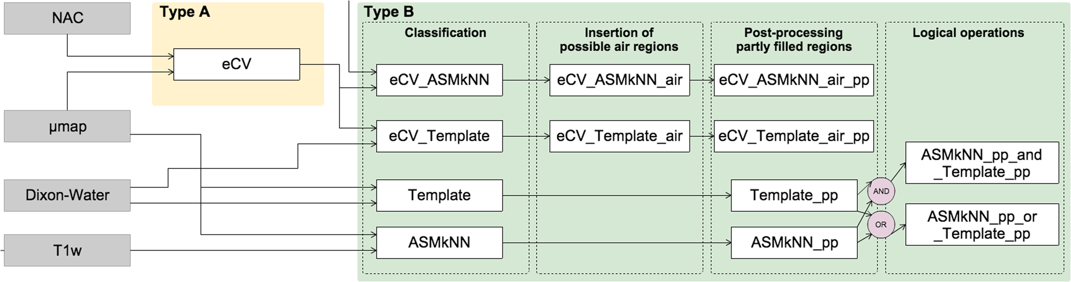
4.1.2.

Artifact 2 [Fig. 2(b)]

The method eCV_ASMkNN_air_pp succeeded in correcting 92% of the artifact volume for patients with artifact 2, but with a relative low-precision score of only 0.34.

4.2.

Type B Artifacts

4.2.1.

Artifact 3 [Fig. 2(c)]

All proposed methods were able to correct the entire artifact area in all patients with artifact 3. The highest precision (0.95) was achieved with the method ASMkNN_pp_and_Template_pp. The method incorrectly filled part of the maxillary sinuses in two patients.

4.2.2.

Artifact 4 [Fig. 2(d)]

For artifact 4 the method Template_pp had the highest recall score, but when looking at the $F 1$ -score, which is a combination of precision and recall, the method ASMkNN_pp_and_Template_pp again achieved the best score (0.96).

The correction method eCV was not applied to the type B artifacts in these results as it was meant for surface breaching artifacts only. Applying the method to the ground truth $μ$ -maps of the 25 patients resulted in an incorrectly filled volume of $5.3 \pm 5.9 mL$ mainly located at the nose. The error is similar to the overestimations observed when correcting the type A artifacts.

5. Discussion

Ignoring metal implant-induced artifacts results in the PET images being biased, a problem previously reported by several authors.⁵^,⁷ No satisfactory solution is available today.⁹ Existing methods do not address dental area specifically, and methods based solely on a mapping from MR data⁴^,²³^,²⁴ will fail since the MR signal is corrupted in areas with susceptibility artifacts. Atlas-based methods depend on a robust nonlinear registration in order to correct the artifacts breaching the anatomical surface, and furthermore, the registration is challenged by the lack of MR signal at the contour we wish to find. This study proposes a new fully automatic approach for correcting artifacts caused by dental implants, which combines the use of existing, modified, and new algorithms. Our approach successfully corrects the attenuation maps over the dental area in patients without extreme abnormal anatomy.

5.1.

Type A Artifacts Breaching the Anatomical Surface

The contour delineation method uses the readily available NAC-PET image since this type of image usually has high photon counts at the borders of the image, making the edge visible even when using tracers with limited uptake outside the brain. The method would not work with area-specific tracers without uptake at the edges; however, such tracers are not yet commonly used.

The method introduces a bias at the nose where the amount of noise is high. The effect of this error is negligible in the PET images after AC in areas outside the nose ( $< 1 %$ ), but is larger in areas close to the nose. The incorrectly inserted volume had an average size similar to a type B artifact. The precision score is highly influenced by the size of the original artifact. This is the reason for the large differences between precision scores of artifact 1 and 2. There is always a tradeoff between over- or under-correcting the artifact. As an example, we increased the amount of erosion performed by the postprocessing method on eCV_ASMkNN_air_pp. This increased the precision score of artifact 1 from 0.74 to 0.94, and of artifact 2 from 0.34 to 0.83, but resulted in a recall score of 0.8 (compared to 0.96) for artifact 1, and 0.73 (compared to 0.92) for artifact 2. In this study, we preferred to correct the artifact fully and thereby erroneously overestimate the contour in areas that do not affect the PET images.

The automatic parameter selection appears robust. The lookup table, which converts the artifact size to actual parameters, has proved successful in our validation. Regularizing the parameters keeps the contour relatively smooth between slices.

5.2.

Type B Artifacts Within the Anatomical Surface

For the differentiation between air-regions and artifacts within the body, we propose a combination of two methods. A template approach with a map of possible air-regions, similar to Ref. 4, and a method built on ASM and kNN.

Our template method offers improvements over Ref. 4 by handling artifacts that are connected to the anatomical air-regions. The accuracy of the method relies on the performance of the affine alignment to the template. The precision of the method is reduced with inaccurate alignment.

To reduce the effect of inaccurate alignment, we propose to represent the potential artifact area by using ASM and kNN. The landmarks are placed in the anatomical T1-weighted MR image typically acquired in the head/neck and brain imaging protocols. The landmarks are placed on the midsagittal slice on the T1w images, since they include the largest section of dental area. It is sufficient to represent the landmarks in two-dimensional (2-D). We tested the method using two additional landmarks placed in each of the pupils, making it a 3-D shape. This extension did not improve the result of the classifier over the presented results using a 2-D shape. The method is able to approximate landmarks placed in signal voids, due to the robustness of ASM. Due to the majority vote after kNN, the classification is robust to some landmark misalignment.

The method incorrectly filled the bottom part of the sinus in two patients. This was due to the initialization of the mean shape being placed too far from the final position. A larger training set and better alignment of the T1w images would be beneficial.

5.3.

Combination of Methods

The reinsertion of air-regions is only an approximation since real borders of the air-region are occluded by the artifact. The number of incorrectly filled voxels was reduced by a factor 2 when using the hole correction method. The misclassified area in the air-regions (5.3 mL) is negligible compared to the original artifact size (artifact 1 mean: 228 mL).

The method ASMkNN had significantly lower precision compared to Template before postprocessing. This is due to resolution differences between the $μ$ -map and the T1w image, which is compensated for by the postprocessing step investigating partly filled signal voids (Template_pp and ASMkNN_pp). Resolution differences are not an issue in the Template method as the $μ$ -map and the DIXON-water image share the same resolution.

Separately, ASMkNN_pp had better or similar $F 1$ -scores compared to Template_pp, thus using the intersection of the two further lowered the number of false positives, as expected.

Specialized multispectral MR sequences for imaging near metal, such as UTE-MAVRIC sequences,²⁵ help improve the overall quality of the MR images. However, artifacts remain in metal, and the performance of multispectral sequences in the context of AC has not been studied on a larger patient cohort. In an eight patient study by Ref. 26, the authors develop a segmentation-based method using intensity thresholding on a high-resolution MAVRIC sequence applied in the oral area. Even though the authors present a significant decrease in artifact size, parts of the artifacts still remain. Our method could still be applied after such multispectral sequences for further correction.

The method does not require prior knowledge about the type of artifact (A or B), nor the possible presence of an artifact. The method runs both correction methods on all patients. Running the method on a patient without artifacts would only result in changes to the PET image that are similar to the bias introduced by this method ( $< 1 %$ outside the nose). In a clinical setup, the correction method should therefore run on all patients after the acquisition of the DIXON attenuation map and the emission data, but prior to reconstruction of the emission data with the attenuation map. An offline reconstruction is also possible if access to modification of the clinical protocols is not available.

This study used simulated artifacts superimposed on patients without dental artifacts. This means no true signal void in the MR-images Dixon-water and T1w exists, which is obviously an advantage for the registration steps used in our method. The frequency of the artifacts, and the performance of the method applied to patients with real artifacts, was assessed in a separate study.¹⁴ Here, we found that out of 339 patients inspected, 148 had dental artifacts of varying sizes. The method proposed here was applied to correct for the artifacts, and after manual inspection of each patient we found that the artifacts had been corrected. The use of artificial voids in this study allowed us to quantify the improvement, something that is not possible when using real patient data.

The method was developed and evaluated using Dixon images, where artifacts tend to pose the greatest challenge for the method, but is not limited to correction of dental artifacts in the Dixon $μ$ -map. Since it has been shown that the method performs well here, it will also perform well using different AC maps with smaller artifacts. Directly substituting the Dixon maps with ones derived from ultrashort echo time (UTE) sequences,²⁷ or any other attenuation map, is possible without modifying the method, as a mask is created during the method, from all tissue values above the LAC representing air.

6. Conclusion

We addressed the previously unsolved problem of correcting for metallic dental implant induced signal voids in PET/MR with a fully automatic approach. The approach solves the problem with high accuracy as shown both visually and quantitatively in our evaluation on $4 \times 25$ patients. The approach uses only images available in all PET/MR head/neck and brain imaging protocols, and is therefore applicable to all patients who do not have abnormal anatomy.

Acknowledgments

The PET/MR scanner at Rigshospitalet was donated by the John and Birthe Meyer Foundation.

References

1.

B. J. Pichler et al., “PET/MRI: paving the way for the next generation of clinical multimodality imaging applications,” J. Nucl. Med., 51 (3), 333 –336 (2010). http://dx.doi.org/10.2967/jnumed.109.061853 JNMEAQ 0161-5505 Google Scholar

2.

G. Delso et al., “Performance measurements of the Siemens mMR integrated whole-body PET/MR scanner,” J. Nucl. Med., 52 (12), 1914 –1922 (2011). http://dx.doi.org/10.2967/jnumed.111.092726 JNMEAQ 0161-5505 Google Scholar

3.

A. Martinez-Möller et al., “Tissue classification as a potential approach for attenuation correction in whole-body PET/MRI: evaluation with PET/CT data,” J. Nucl. Med., 50 (4), 520 –526 (2009). http://dx.doi.org/10.2967/jnumed.108.054726 JNMEAQ 0161-5505 Google Scholar

4.

I. Bezrukov et al., “MR-based attenuation correction methods for improved PET quantification in lesions within bone and susceptibility artifact regions,” J. Nucl. Med., 54 1768 –1774 (2013). http://dx.doi.org/10.2967/jnumed.112.113209 JNMEAQ 0161-5505 Google Scholar

5.

S. H. Keller et al., “Image artifacts from MR-based attenuation correction in clinical, whole-body PET/MRI,” MAGMA, 26 (1), 173 –181 (2013). http://dx.doi.org/10.1007/s10334-012-0345-4 MAGMEY Google Scholar

6.

C. N. Ladefoged et al., “PET/MR imaging of the pelvis in the presence of endoprostheses: reducing image artifacts and increasing accuracy through inpainting,” Eur. J. Nucl. Med. Mol. Imaging, 40 (4), 594 –601 (2013). http://dx.doi.org/10.1007/s00259-012-2316-4 EJNMA6 1619-7070 Google Scholar

7.

Y. Pauchard, M. R. Smith and M. P. Mintchev, “Improving geometric accuracy in the presence of susceptibility difference artifacts produced by metallic implants in magnetic resonance imaging,” IEEE Trans. Med. Imaging, 24 (10), 1387 –1399 (2005). http://dx.doi.org/10.1109/TMI.2005.857230 ITMID4 0278-0062 Google Scholar

8.

I. Bezrukov et al., “MR-based PET attenuation correction for PET/MR imaging,” Semin. Nucl. Med., 43 (1), 45 –59 (2013). http://dx.doi.org/10.1053/j.semnuclmed.2012.08.002 SMNMAB 0001-2998 Google Scholar

9.

G. Delso et al., “Anatomic evaluation of 3-dimensional ultrashort-echo-time bone maps for PET/MR attenuation correction,” J. Nucl. Med., 55 (5), 780 –785 (2014). http://dx.doi.org/10.2967/jnumed.113.130880 JNMEAQ 0161-5505 Google Scholar

10.

J. Nuyts et al., “Completion of a truncated attenuation image from the attenuated PET emission data,” IEEE Trans. Med. Imaging, 32 (2), 237 –246 (2013). http://dx.doi.org/10.1109/TMI.2012.2220376 ITMID4 0278-0062 Google Scholar

11.

G. Schramm et al., “Influence and compensation of truncation artifacts in MR-based attenuation correction in PET/MR,” IEEE Trans. Med. Imaging, 32 (11), 2056 –2063 (2013). http://dx.doi.org/10.1109/TMI.2013.2272660 ITMID4 0278-0062 Google Scholar

12.

T. Chang et al., “Investigating the use of nonattenuation corrected PET images for the attenuation correction of PET data,” Med. Phys., 40 082508 (2013). http://dx.doi.org/10.1118/1.4816304 MPHYA6 0094-2405 Google Scholar

13.

C. N. Ladefoged et al., “PET/MR imaging of head/neck in the presence of dental implants: reducing image artifacts and increasing accuracy through inpainting,” Eur. J. Nucl. Med. Mol. Imaging, 40 228 (2013). http://dx.doi.org/10.1007/s00259-012-2316-4 EJNMA6 1619-7070 Google Scholar

14.

C. N. Ladefoged et al., “Dental artifacts in the head and neck region: implications for Dixon-based attenuation correction in PET/MR,” EJNMMI Phys., 2 (8), 1 –15 (2015). http://dx.doi.org/10.1186/s40658-015-0112-5 Google Scholar

15.

J. Suh et al., “Minimizing artifacts caused by metallic implants at MR imaging: experimental and clinical studies,” AJR Am. J. Roentgenol., 171 (5), 1207 –1213 (1998). http://dx.doi.org/10.2214/ajr.171.5.9798849 AAJRDX 0361-803X Google Scholar

16.

T. Kaneda et al., “Dental bur fragments causing metal artifacts on MR images,” AJNR Am. J. Neuroradiol, 19 (2), 317 –319 (1998). 0195-6108 Google Scholar

17.

T. F. Chan and L. A. Vese, “Active contours without edges,” IEEE Trans. Image Process., 10 (2), 266 –277 (2001). http://dx.doi.org/10.1109/83.902291 IIPRE4 1057-7149 Google Scholar

18.

T. Cootes and C. Taylor, “Active shape models–their training and application,” Comput. Vision Image Understanding, 61 (1), 38 –59 (1995). http://dx.doi.org/10.1006/cviu.1995.1004 CVIUF4 1077-3142 Google Scholar

19.

C. N. Ladefoged et al., “Correction of dental artifacts within the anatomical surface in PET/MRI using active shape models and k-nearest-neighbors,” Proc. SPIE, 9034 90341M (2014). http://dx.doi.org/10.1117/12.2043779 PSISDG 0277-786X Google Scholar

20.

D. Collins et al., “Automatic 3D intersubject registration of MR volumetric data in standardized talairach space,” J. Comput. Assisted Tomogr., 18 (2), 192 –205 (1994). http://dx.doi.org/10.1097/00004728-199403000-00005 JCATD5 0363-8715 Google Scholar

21.

C. N. Ladefoged, “Automatic correction of dental artifacts in PET/MRI,” (2013). Google Scholar

22.

G. Delso et al., “Cluster-based segmentation of dual-echo ultra-short echo time images for PET/MR bone localization,” EJNMMI Phys., 1 (1), 7 (2014). http://dx.doi.org/10.1186/2197-7364-1-7 Google Scholar

23.

A. Johansson, M. Karlsson and T. Nyholm, “CT substitute derived from MRI sequences with ultrashort echo time,” Med. Phys., 38 2708 –2714 (2011). http://dx.doi.org/10.1118/1.3578928 MPHYA6 0094-2405 Google Scholar

24.

M. Hofmann et al., “MRI-based attenuation correction for whole-body PET/MRI: quantitative evaluation of segmentation- and atlas-based methods,” J. Nucl. Med., 52 (9), 1392 –1399 (2011). http://dx.doi.org/10.2967/jnumed.110.078949 JNMEAQ 0161-5505 Google Scholar

25.

M. Carl, K. Koch and J. Du, “MR imaging near metal with undersampled 3d radial UTE-MAVRIC sequences,” Magn. Reson. Med., 69 27 –36 (2013). http://dx.doi.org/10.1002/mrm.24219 MRMEEN 0740-3194 Google Scholar

26.

I. A. Burger et al., “Hybrid PET/MRI: An algorithm to reduce metal artifacts from dental implants in Dixon-based attenuation map generation using a MAVRIC sequence,” J. Nucl. Med., 56 (1), 93 –97 (2015). http://dx.doi.org/10.2967/jnumed.114.145862 JNMEAQ 0161-5505 Google Scholar

27.

V. Keereman et al., “MRI-based attenuation correction for PET/MRI using ultrashort echo time sequences,” J. Nucl. Med., 51 (5), 812 –818 (2010). http://dx.doi.org/10.2967/jnumed.109.065425 JNMEAQ 0161-5505 Google Scholar

Biography

Claes N. Ladefoged is a PhD student at the Department of Clinical Physiology, Nuclear Medicine, and PET at Rigshospitalet, Copenhagen, Denmark. He received his BSc and MSc degrees, both in computer science, from the University of Copenhagen in 2011 and 2013, respectively. After receiving his degrees, he worked as a research assistant at Rigshospitalet before starting his PhD studies in 2015. His PhD work has its main focus on improving PET/MR attenuation correction.

Flemming L. Andersen received his MSc degree in computer science and his PhD degree in medicine from Aarhus University in 1993 and 2002, respectively. Currently, he is the head of IT and modeling at the PET-Unit at Rigshospitalet, Copenhagen University Hospital.

Sune H. Keller received his MSc degree in IT from ITU Copenhagen, Denmark, in 2004, and his PhD degree in computer science from the University of Copenhagen, Denmark, in 2007, where he also worked as a postdoc until 2008. Since 2008, he has worked at Rigshospitalet, University of Copenhagen, as a computer scientist in molecular imaging conducting development, research, and clinical application of PET/MR and PET/CT and corunning the HRRT users software project.

Thomas Beyer received his MSc degree in physics from the University of Leipzig and his PhD degree in medical physics from the University of Surrey in 1995 and 2000, respectively. He received his postdoctoral degree in 2006 in experimental nuclear medicine and became a teaching professor at the Medical Faculty, University of Duisburg-Essen. Since March 2013, he has been a full professor of physics of medical imaging at the Medical University of Vienna, where he is also a deputy director of the Center for Medical Physics and Biomedical Engineering.

Ian Law received his MD, PhD, and DMSc degrees in 1991, 1997, and 2007, respectively. He has worked as a full professor at the University of Copenhagen, Faculty of Health and Medical Sciences since 2014 and as chief physician at the Department of Clinical Physiology, Nuclear Medicine, and PET at Rigshospitalet, Copenhagen, Denmark, since 2005.

Liselotte Højgaard is the chair of the Department of Clinical Physiology, Nuclear Medicine, and PET at Rigshospitalet and professor at the University of Copenhagen and the Technical University of Denmark. She has published 200 peer-reviewed publications. She is the chair of the Danish National Research Foundation, and the EU Advisory Board, Horizon 2020 Health. She is the member of the Conseil d’Administration, INSERM, France, the Royal Danish Academy of Sciences and Letters, and the Danish Academy of Technical Sciences.

Sune Darkner received his MSc degree in applied mathematics in 2004 and founded a software company building databases for the telecommunication industry. He received his industrial PhD degree in “shape and deformation analysis of the human ear canal” in 2009 from the Department of Informatics and Mathematical Modeling at the Technical University of Denmark. Currently, he is an assistant professor in medical image analysis at the Department of Computer Science, University of Copenhagen.

Francois Lauze studied mathematics at the University of Nice-Sophia-Antipolis in France, where he received his PhD in algebraic geometry in 1994. He moved to Denmark and and was awarded another PhD in 2004 at the IT University of Copenhagen. Since 2012, he has been an associate professor at the Department of Computer Science, University of Copenhagen. He works primarily with variational and geometric methods in image analysis and medical imaging.

CC BY: © The Authors. Published by SPIE under a Creative Commons Attribution 4.0 Unported License. Distribution or reproduction of this work in whole or in part requires full attribution of the original publication, including its DOI.

Citation Download Citation

Claes N. Ladefoged, Flemming L. Andersen, Sune H. Keller, Thomas Beyer, Ian Law, Liselotte Højgaard, Sune Darkner, and Francois Lauze "Automatic correction of dental artifacts in PET/MRI," Journal of Medical Imaging 2(2), 024009 (9 June 2015). https://doi.org/10.1117/1.JMI.2.2.024009

Published: 9 June 2015

Access the abstract

JOURNAL ARTICLE
12 PAGES

DOWNLOAD PAPER SAVE TO MY LIBRARY

GET CITATION

CITATIONS

Cited by 11 scholarly publications and 1 patent.

Explore citations on Lens.org

KEYWORDS

Image segmentation

Signal attenuation

Magnetic resonance imaging

Positron emission tomography

Metals

Nose

Image processing algorithms and systems

1.

Introduction

Fig. 1

2.

Materials

2.1.

Patients and Imaging Protocol

2.2.

Construction of Artifact μ-maps

Fig. 2

3.

Methods

3.1.

Type A Artifact Correction

Fig. 3

3.1.1.

Chan–Vese segmentation

Eq. (1)

3.1.2.

First erosion of segmented image

3.1.3.

Postsegmentation

Eq. (2)

Table 1

Fig. 4

Algorithm 1

3.1.4.

Second erosion of segmented image

Fig. 5

3.2.

Type B Artifact Correction

3.2.1.

Template with mask

Fig. 6

3.2.2.

Active shape models

Fig. 7

Fig. 8

3.2.3.

k-nearest neighbors

Eq. (3)

3.3.

Combining Correction Methods

3.3.1.

Postprocessing on partly filled signal voids

3.3.2.

Reinsertion of actual air-regions

Fig. 9

Fig. 10

3.4.

Quality Measures

4.

Results

4.1.

Type A Artifacts

4.1.1.

Artifact 1 [Fig. 2(a)]

Fig. 11

Table 2

4.1.2.

Artifact 2 [Fig. 2(b)]

4.2.

Type B Artifacts

4.2.1.

Artifact 3 [Fig. 2(c)]

4.2.2.

Artifact 4 [Fig. 2(d)]

5.

Discussion

5.1.

Type A Artifacts Breaching the Anatomical Surface

5.2.

Type B Artifacts Within the Anatomical Surface

5.3.

Combination of Methods

6.

Conclusion

Acknowledgments

References

Biography

Construction of Artifact $μ$ -maps