
|
|
1.IntroductionOsteoarthritis (OA) is a major cause for reduced quality of life worldwide, with around 12% of people of 60 years or older suffering from some degree of pain and reduced function in the major load-bearing joints. Due to population aging and an increase in obesity, the prevalence is estimated to double from 2000 to 2020.1 Currently, no effective treatments beyond pain relief are approved, despite several large phase III trials. The lack of successful trials may partly be due to a lack of disease understanding, since OA is a heterogeneous disease affecting multiple tissues,2 and partly due to insensitive study markers. The current food and drug administration (FDA) approved efficacy marker is joint space width measured from radiographs—at best a surrogate marker for cartilage loss, but confounded by influences from meniscus and synovial fluid. The recent recommendation from the Osteoarthritis Research Society International (OARSI) FDA task force is to include cartilage loss measured from magnetic resonance imaging (MRI) as a primary outcome efficacy marker.3 Quantitative analysis of cartilage morphometry from MRI is a demanding task. Manual segmentation by a trained expert requires approximately an hour per scan per desired compartment to be included. A typical phase III clinical trial can include 5000 scans (1000 participants, 3 visits, 1 to 2 knees per visit) and cover the main knee cartilage compartments (medial and lateral tibial, femoral, and patellar cartilages—see Fig. 1 for illustration); ideally requiring around 25,000 expert hours of interaction. The large epidemiological osteoarthritis initiative (OAI) study4 includes 4796 subjects with MRI and ultimo 2013 six main visits with a total of 24,885 MRI visits and approximately 50,000 scans of left and right knees for a given sequence. Including five cartilage compartments, around 250,000 expert interaction hours would be needed corresponding to around 125 working years. This reader bottleneck makes comprehensive analysis infeasible—if based on manual segmentation. Furthermore, more advanced three-dimensional (3-D) morphometric markers, such as cartilage surface smoothness5 or joint congruity,6 will suffer from the inter-slice discontinuity artifacts caused by slice-wise delineation. Finally, inclusion of additional structures beyond cartilage only increases the quantification challenge. Fig. 1Visualizations of fully automatic segmentations. (a) A Center for Clinical and Basic Research (CCBR) validation scan with the Tibia bone and the medial tibial and medial femoral cartilages segmented. (b) An osteoarthritis initiative (OAI) validation scan with medial/lateral tibial/femoral cartilages in golden colors, and patellar cartilage and medial/lateral menisci in red/green/blue. The tibial cartilages are mostly hidden behind other compartments. (c) A SKI10 validation scan with Tibia and Femur bones and medial/lateral tibial/femoral cartilage subcompartments. Note that for SKI10 evaluation, the medial and lateral cartilage subcompartments were combined.  Several promising attempts for automatic segmentation of knee MRI have been proposed. Early approaches applied slice-wise two-dimensional (2-D) active shape models (ASM)7 and 2-D active contours8 and demonstrated the feasibility of automated cartilage segmentation. Another early approach used semi-automatic 2-D geodesic snakes for bone segmentation.9 A semi-automated 3-D method based on a registration-based spatial prior and -nearest neighbor (-NN) voxel classification10 demonstrated proof of concept on a few cases as early as 1998. Later, an effective semi-automated 3-D graph-based approach was proposed.11 Still, a 2006 review concluded that no fully automatic approaches existed.12 The first fully automatic method for cartilage segmentation was published in 200513 and later refined in 2007 based on supervised voxel classification with Dice volume overlaps of 0.80 for medial tibial and 0.77 medial femoral cartilages.14 Also in 2007, a method for fully automatic knee bone segmentation appeared.15 Recently, as also evaluated at a medical image computing and computer-assisted interventation (MICCAI) workshop entitled “Segmentation of Knee Images 2010” (SKI10), more automated methods have emerged.16 The current top-scoring method at SKI10 (as of March 2015) is fully automatic based on an active appearance model, where the bone shape models have been built using the minimum description length approach for optimizing correspondences between point distribution models, with average tibial and femoral cartilage volume overlap errors at 23.4% and 23.9%.17 The second scoring at SKI10 is also based on bone shape models, but the cartilages are segmented using a multiobject graph optimization method that results in cartilage overlap errors of 25.8% and 26.4%, respectively.18 Unfortunately, the SKI10 results are difficult to interpret since the cartilage segmentations are only evaluated in central load-bearing regions—excluding the sheet peripheries that are often very challenging.19 In general, comparisons across populations are obviously problematic. In other medical image segmentation tasks, a lot of attention has been given to registration-based approaches. Nonlinear registration methods have matured allowing elastic, diffeomorphic, and other geometric transformation classes,20 and the implementations are now feasible in terms of computation time. However, for joint segmentation, it is not obvious to follow this trend. First, joints are a mixture of rigid and soft tissue, meaning that standard elastic registration approaches may be too flexible. Second, the important cartilage compartments are so small that a standard registration objective function may implicitly prioritize registration accuracy in the bones rather than the cartilages. Finally, cartilage denudation results in topological changes that are problematic in diffeomorphic registration models. It would appear that dedicated methods are needed for robust and accurate joint registration—such as articulated-rigid bone registration followed by locally elastic registration in cartilage areas. The third-ranking SKI10 method actually applies a multiatlas nonrigid registration approach to produce an initial segmentation that is used as an input to a graph-cut method, resulting in cartilage overlap errors of 28.3% and 27.6%, corresponding to Dice 0.677 and 0.719 for tibial and femoral cartilages (from UPMC, previous version presented21). The fifth-ranked method22 also applies multiatlas registration using patch-based label fusion (previously demonstrated to be very applicable for brain MRI segmentation) followed by a specialized three-class classification. This demonstrates the potential for registration-based methods, but also the need for combination with other approaches. The objective of this paper was to introduce and evaluate the knee image quantification (KneeIQ) framework for fully automatic segmentation of knee joints from MRI that combines some of the appealing aspects from the previous approaches. We used a voxel classification framework heavily inspired by Folkesson et al.,14 but combined it with a new multiatlas preregistration step. The rigid preregistration allowed the selected classification features to be more specific to the individual structures since the majority of the background was effectively identified and the structures were better aligned. The framework allows varying structure sets and can be used for different collections with different configurations of available bone/cartilage/meniscus compartments training data. We demonstrated the proposed framework for segmentation of low- and high-field knee MRIs from three cohorts and evaluated it against manual segmentations. The extensive evaluation included fully automatic segmentation of 1907 knee MRIs. Example segmentations from each cohort are visualized in Fig. 1. The validation demonstrated a performance similar to manual segmentations and equal to or better than other automated methods in terms of accuracy and precision. 2.MethodsThe methods section includes descriptions of the cohorts, the segmentation framework, and the experiments. 2.1.Knee MRI CollectionsWe used three collections of knee MRI from the Center for Clinical and Basic Research (CCBR), the OAI study, and the SKI10 challenge. The collections included scans with manual segmentations that we used for training and validation. The relevant ethical review boards approved the studies. The collections substantially differed in scanner type, scan quality, and disease severity as described below. The scanner specifications and the analyzed anatomical structures are described in Table 1 and the populations are summarized in Table 2. Table 1Study descriptions in terms of scanners, sequences and available manual annotations.
Table 2Cohort population characteristics for training and validation subpopulations from CCBR and OAI. The SKI10 collection includes 60 training, 40 test scans, and 50 validation scans, but the population characteristics are unavailable.
2.1.1.CCBR Low-Field MRI StudyThe low-field MRI collection was from a community-based study conducted at CCBR. The cohort was from the greater Copenhagen area with a large age span and a mix of healthy and subjects with mild to advanced radiographic OA. The scans were acquired using a low-field MRI scanner dedicated for extremities. A subset of the knees were rescanned a week after the baseline scan—which allowed scan-rescan precision evaluation. A large set of manual segmentations of medial tibial and femoral cartilages were made by a trained radiologist using slice-wise outlining. This set including repeated segmentations on the subset of the scans, which were also rescanned. For this subset, the radiologist manually segmented all first scans, then all second scans, and then the first scans again. Therefore, both intra-scan and scan-rescan radiologist performances are available to use as a yardstick for the evaluation of the automatic segmentation framework. For the training scans, manual segmentation of the Tibia bone is also included. The validation included all CCBR MRI scans with manually segmented cartilages. 2.1.2.OAI High-Field MRI CohortThe OAI is a large, NIH-funded study made in collaboration among OARSI, National Institute of Arthritis and Musculoskeletal and Skin Diseases, industrial partners, and others. The study is unique in the size as well as the duration with 4796 subjects that have been followed with yearly visits since 2004. The OAI data were obtained from the OAI database, which is publicly available in Ref. 4. We used dataset 0.E.1. For a subset of 88 subjects, the OAIs have made a collection of semi-manual segmentations provided by iMorphics publicly available. Since these segmentations were made using a semi-automated annotation tool with some implicit boundary bias, they may not quite be golden standard radiologist segmentations, but they are applicable for the validation of automated methods. The subcohort resembles a typical OA clinical trial population with moderate or severe OA [Kellgren and Lawrence score (KL) 2 or 3]. The iMorphics segmentations include medial and lateral tibial cartilages, femoral and patellar cartilages, and medial and lateral menisci. To be consistent with the CCBR data, we split the femoral cartilage into medial and lateral subcompartments by manually selecting the slice where the femoral notch is approximately deepest at the center between the two condyles. Further, cartilage volume measurements from other groups, VirtualScopics and Chondrometrics, are publicly available for validation. The VirtualScopics segmentations were from a semi-automated method,23 whereas the Chondrometrics were done by expert manual readers. The validation included all OAI scans with such scores for the first visit. 2.1.3.SKI10 High-Field MRI CollectionThe segmentation of knee images challenge was part of the workshop at the 2010 MICCAI conference. The purpose was to allow comparative evaluation of segmentation methods.16 The collection includes 100 scans with manual segmentations for training and testing. Among the 100 training scans, 40 also have labels for a region of interest (ROI) inside the central load-bearing regions of the medial and lateral tibio-femoral compartments. Another 50 validation scans without publicly available manual segmentations are used for the actual challenge evaluation. Currently, 18 teams have submitted results that are publicly available in Ref. 24. The scans are from patients undergoing knee surgery and were provided by Biomet Inc., together with manual segmentations. The segmentations were used during surgery planning and are different from the typical segmentations used for clinical studies (like the CCBR and OAI studies). They were made to be accurate in the central regions, but it is somewhat arbitrary whether the surfaces around the periphery of the cartilage compartments are marked as bone or cartilage (this is not important prior to total knee replacement). Therefore, the SKI10 challenge only evaluates the cartilage segmentations inside smaller ROIs at the centers of the load-bearing regions. The scanners and MRI sequences cover a very large variety (see Table 1); therefore, the scans in the collection are not homogeneous like the CCBR and OAI collections. Since the knees are selected for surgery, they typically have progressive OA, but no information is available regarding KL, age, body mass index or the like. The SKI10 scans were preprocessed as follows:
2.2.Automatic Segmentation FrameworkThe proposed segmentation framework combines rigid multiatlas registration with voxel classification in a multistructure setting (see Fig. 2 for illustration of the workflow). The voxel classification step includes an ROI analysis and a feature selection for each structure. This is a generalization of the method proposed by Folkesson et al.14 that was implemented for the two medial cartilage compartments. Here, we generalized to arbitrary compartments and added the registration step to improve the performance. Fig. 2Flowchart of the quantification steps. The multiatlas registration, region of interest (ROI), and feature computation steps are performed both during training (top) and scoring (bottom). The training phase results in the transformations for the training scans, the ROI definitions, and the selected feature sets—these parameters are used during scoring of “unseen” scans. 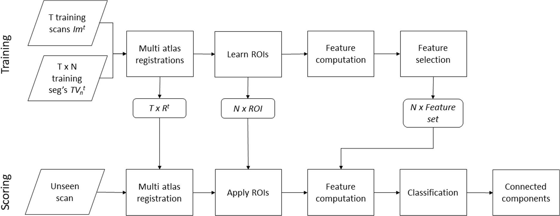 2.3.Training DataWe assumed the existence of training scans , for which structures have been (manually) outlined, forming a set of ground-truth segmentations. An example scan with manual segmentation is illustrated in Fig. 3. These were represented by training volumes with , , where each gave the presence of structure . This allowed for binary segmentations with values or for partial volumes with values [0,1]. Overlapping structures were allowed. The scans were assumed to be of dimension , where . Fig. 3Scan, manual segmentation, and automatic segmentation for a validation scan from the OAI collection. Three sagittal slices are shown going through the centers of the (a) tibial medial cartilage, (b) patellar cartilage, (c) tibial lateral cartilage. The scan slice (left) is given with the manual (center) and the automatic segmentations (right). The Dice volume overlaps for the example were between 0.84 and 0.91 for the tibial and femoral cartilages, 0.76 for the patellar cartilage, and 0.78 and 0.80 for the menisci. 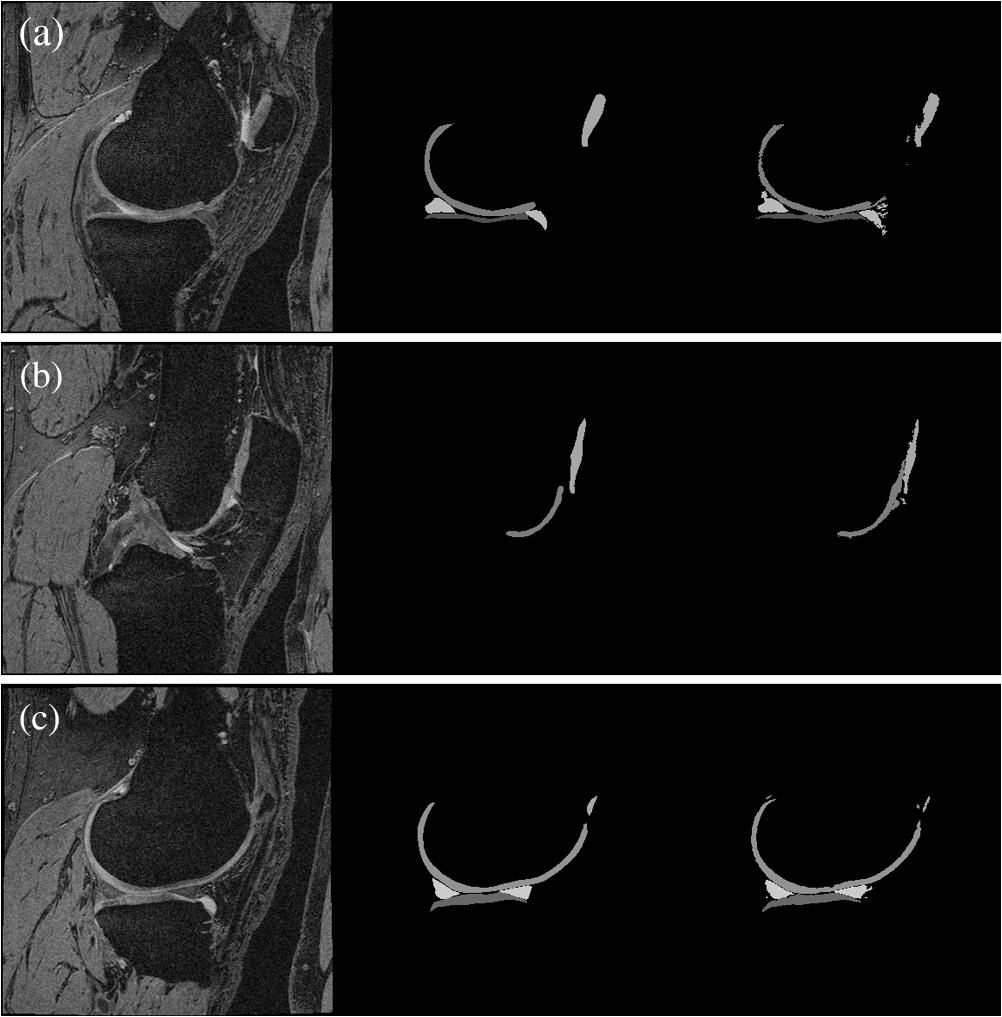 2.4.Multiatlas Rigid RegistrationThe aim of the registration step was to produce a transformation from a given scan to a training space center. As explained below, this allowed determination of the ROI for each anatomical structure and transformation of scan features to a common feature space. The effect of the inter-subject alignment from the registration step is illustrated in Fig. 4. Fig. 4The effect of multiatlas registration illustrated for scans in the CCBR training collection. The manual segmentations for the three structures (Tibia, medial tibial cartilage, and medial femoral cartilage) are accumulated in the three color channels of an RGB picture and shown in a slice in the middle of the medial compartment. (a) This is done before and (b) after registration. The intensity in each pixel can be interpreted as a spatial prior for each structure. (a) Before registration, these values ranged from 0 to 1.00, 0.34, and 0.28 for the three structures. (b) After registration, they ranged to 1.00, 0.86, and 0.73.  We represented a transformation as a vector including elements for translations, for Euler angle rotations, and 1 for isotropic scaling. By allowing scaling, the registration is not mathematically a rigid transformation, but a similarity transformation. We registered two given scans by maximization of normalized mutual information25 (NMI) using L-BFGS optimization.26 The optimization was performed in two steps with Gaussian blurring of the scans at a coarse scale and then at a fine scale. During training, each training scan was registered to all training scans , , where the optimization was initialized by the translation implied by the center of masses (CoMs) of the manual segmentations of a specified structure. This initialization ensured a robust estimate for all training scans. From the resulting similarity transformations , the transformation to a training space center was defined as the element-wise median. The median transformation for training scan was denoted . When segmenting a (new) scan , the scan was registered to all training scans, but with no initialization, resulting in similarity transformations . The compositions provide an estimate of the transformation to the training space center via a training scan. Due to inter-subject variation, scanner noise, and optimization failures, the estimates will not be identical; however, the element-wise median of the compositions defined a robust estimate of the final multiatlas transformation for the given scan to the training space center. We experimented with more sophisticated definitions of the typical transformation than the element-wise median—specifically atlas selection based on the NMI score and with a geometric transformation based on Fletcher’s principal geodesic analysis.27 However, none of these experiments improved the performance, therefore, we used the simplest approach. Note that since the angle coordinates represent rotations; they are typically close to zero (and definitely between and ) and, therefore, have no angle wrap-around challenges. 2.5.Structure-Wise Regions of InterestBoth in terms of computational efficiency and classifier specificity, it is advantageous to only train and apply a classifier on the region surrounding the structure of interest. We learned a simple rectangular ROI in the registered scans for each structure. Figure 5 illustrates the resulting ROIs learned from the OAI training data. Fig. 5Visualization of the learned regions of interest (ROI) for the OAI training collection. For each structure, the coordinate extrema after multiatlas registration are added a margin to cover feature filter support. These resulting bounding boxes are shown from sagittal/coronal/axial views. Each structure is only trained and segmented inside the ROI.  Specifically, we defined a structured ROI as the coordinate extrema encountered in the registered training scans with an added margin of 5% of the scan’s size in each direction. Thus, the structures with margin for feature filter support were inside the ROI. 2.6.Voxel Classification FeaturesThe features used for the voxel classifier were very similar to the set previously used by Folkesson et al.14 As potential features, we used the N-jet28 including Gaussian derivatives up to order 3, and nonlinear combinations of these including the Hessian and structure tensor eigenvectors and values. Also, intensity and position were included. All nonposition features were computed at scales of 0.6, 1.2, and 2.4 mm. This gave a 178-dimensional space of potential features. The position and Gaussian derivative features for a given scan were transformed using the similarity transform from the multiatlas registration step. Each individual feature was translated and scaled such that the values for the training collection had mean 0 and standard deviation 1. 2.7.Training Voxel SamplingA large set of training voxels are desired to ensure classifier generalizability. However, for practical computations, the computer memory is limiting the training size. Also, it is desirable to sample the training voxels to be specific to the classification task at hand. Particularly with small/thin structures like cartilages, it is desirable to include many structure voxels, relatively many near-structure background voxels, and fewer voxels from the background far away from the structure in the training scans. We applied a simple sampling scheme with a constant sampling density inside each structure, another density in the background and a linear transition in density in a narrow margin around each structure. The exact sampling densities were calculated such that the training data for each structure would be suitable for execution on a standard laptop computer. Each voxel from the training scan included in the training data was attributed with the local sampling density . 2.8.Feature SelectionWe used floating forward feature selection29 optimized on the sampled training voxels for defining the actual set of features used for each structure. The Dice overlap on the sampled training voxels was used as an optimization criterion. With the sampled training voxels, the overlap contribution must be inversely weighted with the local sampling density. For a given feature set and a given hard classifier returning 0 or 1 indicating membership for structure , with sampled training voxels : The overlap was evaluated using leave-one-scan-out such that the evaluation of sampled feature voxels from a given scan only included training voxels from the other scans. To encourage sparse feature sets, a penalty of 0.001 per feature was added to the Dice overlap in the feature selection objective function. This avoids the addition of several additional features with only marginal improvement on the training collection—therefore, the generalization to the validation set was potentially improved. Typically, the feature set for each knee structure classifier became 10 to 30 dimensional. 2.9.Structure-Wise ClassificationThe above feature selection and sampling strategies can be used for any classifier. Like Folkesson et al.,14 we applied a -NN classifier to allow for multimodal distributions with no assumptions on the feature distributions that will arise from the different structures. Other nonlinear classifiers such as support vector machines, random forest, or convolutional neural networks could also be appropriate and are likely computationally more efficient. For -NN to become a hard classifier, a threshold on the number of neighbors is needed. For each structure, this threshold () was determined during training to optimize the Dice overlap score for a given feature set. The classification strength was defined as the -NN count minus such that 2.10.Multistructure Segmentation of a New ScanAbove, we trained independent structure-wise classifiers to allow dedicated feature selection for each structure and simple generalization to multiple structures. When segmenting an unseen scan, we first performed the multiatlas registration step resulting in the atlas transformation (element-wise median of ). This transformation was applied to each trained structure ROI, defining a bounding box for each structure in the scan. The trained, structure-specific features were computed within the ROIs and we applied each structure-classifier independently. For computational efficiency, we used the sparse sample-expand and sample-surround sparse classification methods.30 These methods essentially aim to only classify voxels that are relevant for the segmentation in order to improve computational efficiency. The sample-expand algorithm is a region-growing algorithm that is initiated in many randomly defined seed voxels in the scan. For each seed, the structure classifier is used and the region is grown if the classifier determines the voxel to be inside the structure. This growing continues to neighbor voxels in a breadth-first manner until a connected component is formed. The number of seed voxels is defined to ensure that all components of a suitable size are hit by a seed point (i.e., the probability of missing a component is below ). This sample-expand region growing is very effective for small/thin structures since the majority of the scan voxels are not classified. For large, compact structures, the sample-surround algorithm does not expand in all directions, but rather makes a line search to the object boundary and then only classifies voxels necessary to outline the structure boundary. We apply sample-expand sparse classification for cartilages/menisci and sample surround for the bones. For each structure, the one-versus-all -NN classifier resulted in classification strengths in the classified voxels. The voxels that were not visited by the sparse classification methods were assumed to have strength -1. These structure-wise strength maps were combined to form a single map of class labels by assigning each voxel to the structure with the highest strength. This was followed by a largest connected components step including the largest components to exclude small, spurious components. 2.11.Experimental SetupGiven the annotated training data, the above framework is fully automatic. The following set of fixed parameters was used for all experiments. The rigid registration was optimized at blurring scales 5 mm and then 1 mm using 64 histograms bins in the NMI computation. NMI was computed using a regular grid of evaluation points with 2-mm spacing, except the 15% outer margin of the scans was ignored to avoid nonoverlap artifacts. The voxel classification features were computed at blurring scales 0.6, 1.2, and 2.4 mm. During feature selection, the training voxel sampling was performed with densities (as outlined above) such that the training data for each structure approximated 250 MB assuming a resulting 30-dimensional feature vector. The narrow margin around each structure was set to 4 mm (approximately double the thickness of a cartilage sheet). The -NN classifier was used with and approximation parameter in the approximate nearest neighbour implementation.31 The largest connected components step was performed to include components with a volume above 15% of the volume of the largest component. To investigate the effect of the multiatlas registration step, the entire framework was evaluated without this step. Thereby, the framework becomes essentially equivalent to the original Folkesson framework.14 Unlike Folkesson, the nonregistration framework still allows an arbitrary set of structures and there are implementation differences, but the basic methodology is very similar. We denote this variant Folkesson07. 2.12.Statistical AnalysisSegmentation accuracy was evaluated by the Dice volume overlap score where segmentations were available. Where only volume scores were available, accuracy was evaluated by the Pearson linear correlation coefficient , the absolute agreement intra-class correlation coefficient, and by the median of signed, relative differences (in %). Segmentation precision was evaluated by the root-mean-squared coefficient of variation (RMS CV) of the cartilage volume pairs. This was done both on repeated segmentations of the same scan (intra-scan) and on segmentations of repeated scans from the same subject acquired within a short period (inter-scan). For the SKI10 collection, we used the evaluation metrics defined by SKI10 that combines surface distances measures into a bone score and volume overlap/difference measures into a cartilage score.16 The bone and cartilage scores are both normalized by comparison to inter-reader variation such that a score of 75 matches the performance of the SKI10 expert manual readers. 3.ResultsFrom the CCBR study, the evaluation included MRI scans from 140 knees of which 30 were used for training and 110 for validation. Of the 110, 38 were rescanned a week after the baseline scan. From OAI, the evaluation included the MRI with semi-manual segmentations of which 44 were used for training and 44 for validation. In addition, the validation included 150 MRI with volume scores from VirtualScopics and 1436 with scores from Chondrometrics. Finally, from SKI10, 60 scans were used for training, 40 scans for validation, and 50 scans were sent to SKI10 for challenge validation. In total, 174 MRI scans were used for training and 1733 for validation. The population characteristics are summarized in Table 2. 3.1.Multiatlas Registration EffectsAs illustrated in Fig. 4, the registration step makes the positioning of the structures more consistent. For each structure, this is quantified by the CoM position variation (PV) defined as the mean distance from each CoM to the training collection mean CoM. For the CCBR collection, the cartilage compartment PVs were 8.4 to 9.2 mm before registration and 1.8 to 4.0 mm after registration. For the OAI collection, the cartilage PVs were 8.0 to 9.3 mm before and 2.7 to 5.1 mm after. However, here the tibio-femoral compartments were all close to 3 mm, whereas the patellar was higher at 5.1 mm. Finally, for the SKI10 collection, the cartilage PVs were 7.3 to 10.9 mm before and 3.5 to 4.4 mm after. The ROIs illustrated in Fig. 5 also illustrate a registration effect. For the CCBR collection, the volumes of the tibial and femoral cartilage ROIs were 9%, and 32% of the full scan corresponding to 61 and 79 times the mean volume for each structure. In comparison, for the Folkesson variant without registration, the cartilages ROIs were 23% and 38% of the scan and 147 and 87 times the structure volume. For the OAI collection, the ROI relative volumes were 5% to 6% for tibial/patellar and 14% to 15% for femoral cartilages—corresponding to 45–56 times the structure volumes. 3.2.Segmentation AccuracyThe training and validation segmentations accuracies are shown in Table 3 for the CCBR and OAI collections. For medial/lateral tibial/femoral cartilages, the validation volume overlaps were between 0.804 and 0.866. For patellar cartilage and menisci, they were a bit lower. Table 3Segmentation accuracy for training and validation in the Center for Clinical and Basic Research (CCBR) and osteoarthritis initiative (OAI) collections. Accuracy is given as the Dice volume overlap showing mean±std over minimum/maximum values. The number of knees (n) is given for each set.
For comparison, for the CCBR study the radiologist repeated the manual segmentations for the 38 scans also used for the scan-rescan precision analysis. The intra-operator, intra-scan mean Dice volume overlaps for the medial tibial and femoral cartilages were 0.858 and 0.860. 3.3.Cartilage Volume PrecisionThe intra-scan and inter-scan precision for the CCBR collection is given in Table 4. The radiologist had an intra-scan precision 6% to 7% and a can-rescan precision at 9%. The automatic method had an intra-scan precision of 0%, demonstrating that repeated runs on the same scan reproduced the volume scores, and a scan-rescan precision at 5%. When merging the segmentations for the two medial compartments, the precision was considerably improved for the radiologist, but only marginally for the automatic method. Table 4Precision of cartilage volumes for the 38 scan-rescan knees from the CCBR collection. The intra-scan results are for repeated segmentations on the same scan. The scan-rescan results are for segmentations of different scans acquired approximately 1 week apart. Precision is given as root-mean-squared coefficient of variation (RMS CV).
3.4.Cartilage Volume Comparisons on OAIBoth VirtualScopics and Chondrometrics have cartilage volumes available via the OAI, quantified for 150 and 1436 knees, respectively. For the interested reader, the Biomediq cartilage volume scores are available for the same knees at the Biomediq website.32 Table 5 shows the level of agreement between the KneeIQ quantifications and the alternative methods. Due to differences in subcompartment definitions for the femoral cartilage, only the medial/lateral tibial compartment volumes are included. Table 5Agreement between the automatic knee image quantification (KneeIQ) volume scores and the scores from the independent groups on different subset from the OAI cohort. The table includes number of knees available (n), Pearson linear correlation coefficient (r), absolute agreement intra-class correlation coefficient (ICC) and median signed relative difference (%).
The agreement between KneeIQ and Chondrometrics cartilage volumes is further illustrated by the Bland–Altman plots in Fig. 6. Fig. 6Bland–Altman plots of the agreement between manual Chondrometrics and automatic knee image quantification (KneeIQ) segmentations for the tibial compartments [(a) lateral, (b) medial]. The agreements were evaluated by linear correlations of 0.90 and 0.91 and intra-class correlation coefficients (ICCs) of 0.90 and 0.81, respectively. The measure difference is shown as KneeIQ-Chondrometrics scores implying that KneeIQ overestimated compared to Chondrometrics. The horizontal, dotted lines show steps of a standard deviation above and below the mean. 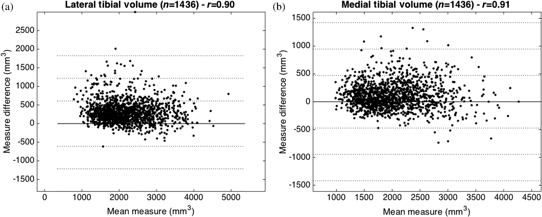 For a subset of 58 knees, the volume scores are available for all four methods. The mutual agreements for this subset are shown in Table 6. Table 6For 58 OAI knees, volume scores are available for all groups. The inter-agreement is given as Pearson linear correlation coefficient (r) and mean signed relative difference (%). Positive differences mean that the method in the left column has higher volumes, on average.
Generally, the correlations are high between all methods, ranging from 0.90 to 0.97. There is a tendency for the automated methods to estimate the volumes higher than the manual scores from Chondrometrics. 3.5.SKI10 EvaluationThe results for the validation on the SKI10 collection are available in Ref. 24. The performance on the training set gave Dice overlap scores of 0.97 for the tibia and femur bones and 0.64 to 0.73 for the cartilage compartments.33 The official scores for the evaluation set include volume overlap errors of 25.9 and 25.7 for the femoral and tibial cartilages, contributing to cartilage scores of 65.4 and 66.7, respectively. The bone scores include RMS surface distances of 1.4 and 1.0 mm for femur and tibia, contributing to bone scores of 63.2 and 61.8. 3.6.Comparison to Folkesson07The importance of the multiatlas registration step was evaluated on the CCBR cohort. The Folkesson07 variant had volume overlaps of 0.823 and 0.772 on the medial tibial and femoral compartments, as compared to 0.839 and 0.804 for the full KneeIQ framework. The scan-rescan precision was 5.6% and 7.8% for Folkesson07 against 4.9% for KneeIQ. 4.Discussion4.1.Previous Results on the Validation CollectionsThe CCBR, OAI, and SKI10 collections have previously been investigated with respect to segmentation and cartilage quantification. On the CCBR collection, Folkesson et al reported results on a fully automatic segmentation of the tibial and femoral medial cartilage compartments, including volume overlap scores at 0.81 and 0.77, respectively, and scan-rescan precision given by mean absolute volume differences of 5.8% and 7.4%, respectively.14 For OAI, several investigations were performed on the sagittal DESS scans. A pilot population of 19 with a mix of healthy and OA subjects were segmented twice unpaired and the precision was evaluated by RMS CV. For cartilage volume, RMS CV was 3.9% and 8.2% for medial and lateral tibia, and 6.2% and 4.6% for posterior medial and lateral femoral subcompartments.34 Another OAI study compared different segmentation methods on the 19 subjects.35 The across-methods pooled RMS CV scores for the DESS scans were 7% for medial and lateral tibial compartments and 6% and 7% for the central medial and lateral femoral compartments. Using OAI scans, a multiobject graph optimization method demonstrated a good segmentation performance on a small subset of 9 scans.36 The volume overlaps were between 0.80 and 0.84 for the cartilage compartments. Recently, an automatic method combining a bone ASM segmentation, a semantic context forest cartilage classifier, and smoothing by a graph cut optimization was presented at a workshop.37 The method was validated on the OAI subcohort with manual segmentations by iMorphics also used in this paper. The Dice volume overlaps for the cartilages were between 0.79 and 0.85. The semi-automated VirtualScopics segmentation method has also been applied to the OAI knee MRI;23 however, no papers with segmentation performance metrics are known. Finally, 19 methods have been evaluated on the SKI10 collection. In the normalized scores where 75 matches an expert, manual reader, the bone scores range from 11 to 77 and the cartilage scores range from 23 to 67. 4.2.Comparison to Previous ResultsThe performance of the Folkesson07 variant was close to the results originally reported by Folkesson. This supports the observed performance improvements due to the new multiatlas registration step. On average for the two medial compartments, the volume overlap improved by 0.024 and the precision improved by 1.8%. Looking at the segmentation accuracy on the OAI cohort, our validation volume overlaps between 0.81 and 0.87 for the medial/lateral tibial/femoral compartments compare well with the best published results and may even be slightly higher. However, for the patellar cartilage, our volume overlap at 0.74 is slightly lower than the best published results. The studies on the 19 OAI subjects suggest that variations around 5% to 6% in tibial and femoral cartilage volume scores are to be expected for scan-rescan experiments using a specific method and around 7% using similar, but different methods. The agreements between the cartilage volumes from our method and the independent methods (Tables 5 and 6) appear to be within this range except for the comparison to Chondrometrics scores in the lateral tibial compartment. Apparently, even if our overestimations compared to the iMorphics segmentations are acceptable around 4 to 5%, the overestimation of iMorphics compared to Chondrometrics of 8% in this compartment resulted in a larger, total overestimation of 14%. Due to the lack of Chondrometrics segmentation masks, this specific discrepancy is difficult to directly investigate. Our validation against a large collection of manual segmentations is similar in spirit to the evaluation by Shan et al.22 They also measure the linear correlation between automatic and manual segmentation volumes. For their 700 scans, the linear correlations were 0.87 for the tibial cartilage and 0.77 for the femoral cartilage. For the 1436 scans in our evaluation, we achieved automatic to manual correlations of 0.90 and 0.91 for medial tibial and femoral cartilages. 4.3.Comparison to SKI10 ResultsOur method performed mediocre for bone segmentation scoring 62.49 and second highest for cartilage segmentation scoring 66.10. 4.4.Segmentation ErrorsVisual inspection demonstrated that the voxel classification independently performed in each voxel resulted in focal fine-scale artifacts in the segmentations (see Fig. 3). Therefore, our results could possibly be improved by a regularization postprocessing step that refines the segmentation boundaries using either local or global shape information. This could be using a multiobject shape model or possibly by a more local regularization process like the graph cut optimization used by Wang et al.37 However, markers that are to be quantified from the segmentations may be robust to these fine-scale details. A cartilage volume marker will likely not be significantly affected and markers that are quantified with explicit or implicit regularization will also be robust to this, such as surface smoothness38 and joint congruity.6 For the OAI collection, our automatic segmentations overestimated the cartilage volumes by 4% to 5% compared to the iMorphics validation scans (see Table 5). Compared to the VirtualScopics, our estimations were, on average, almost equal. Compared to the Chondrometrics volumes, both the iMorphics and our method estimated the numbers to be higher. The plots in Fig. 6 reveal that this overestimation mainly originated from the knee with relatively little cartilage. The availability of semi-manual segmentations for the iMorphics validation set allowed further inspection of the source of the overestimation (Fig. 7). By applying the transformation from the multiatlas registration step, we transformed all segmentation differences to a common reference space. The figure illustrates that some locations were common for oversegmentation (defined as voxels in the automatic segmentation, but not in the validation segmentation, in more than 10% of the 44 cases). This oversegmentation region generally corresponded to the peripheral rim of the cartilage sheets, as illustrated for the medial tibial compartment in Fig. 7. This observation confirmed the conclusion from Williams that segmentation of the periphery is particularly challenging.19 Fig. 7Locations of overestimation in the OAI segmentation. (a) Using the multiatlas registration transformations, the mean shape of the manual segmentations can be visualized, as done for the medial tibial compartment. Likewise, the differences between manual and automatic segmentations can be transformed to the same space. (b) The locations of the volume overestimations are visualized showing the locations that in at least 10% of the OAI validation scans were included by the automatic but not the manual segmentation. This is generally in the periphery of the sheet. These oversegmentation locations are color-coded with the mean distance to the manual segmentation with the range shown in the color bar in mm. The sheet is shown with external left, internal right, anterior up, and posterior down.  For the SKI10 scans, visual inspection revealed bone segmentation errors in the shafts toward the boundary of the scans for the cases with weak image quality. A statistical shape model would be the classical approach to handle this. 4.5.Segmentation of Pathological KneesIt is often assumed that pathological structures are more challenging to analyze than healthy structures due to larger biological variation. The OAI validation population only included KL 2 and 3 knees; however, the CCBR collection allowed analysis of this effect for both automatic and manual segmentations. Specifically, with stratification according to degree of radiographic OA (KL score 0 or 1 versus ) of the CCBR rescan subgroup, the mean Dice overlap scores for our automatic method were 0.843 versus 0.802 for the medial tibial compartment and 0.814 versus 0.780 for the medial femoral compartment. In comparison, the repeated radiologist segmentations had Dice 0.860 versus 0.854 for tibial and 0.870 versus 0.837 for femoral. Therefore, the segmentation accuracy for Dice may be expected to be 0.03 lower for ROA than for healthy tissues, where the effect is slightly larger for the automatic method than for expert manual segmentations. 4.6.Methodology ChoicesThere are several approaches to automatic knee MRI segmentation. Some methods are directly hierarchical starting with a bone segmentation that then aids the (more difficult) cartilage segmentation with features for distance-from-bone or position-relative-to-bone.18,36,38–42 Other methods achieve a similar coarse-to-fine effect by applying atlas-based registration before either nonrigid registration21,40,43 and/or classifier-based segmentation.10,22,43 In general, it appears that integration of global information and local features is essential for solving the challenging problem of segmentation of cartilage on the background of multiple other tissue types. This explicitly or implicitly allows a zoom to several, simpler, local segmentation tasks such as cartilage versus subchondral bone, cartilage versus meniscus, cartilage versus cartilage, and cartilage versus synovial fluid. Due to differences in populations, scanners, sequences, and particularly disease stage, it is challenging to compare segmentation performances across these publications. However, it would appear that tibial/femoral cartilage Dice volume overlaps around 0.85 are attainable with these automatic methodologies. In our methodology, the rigid multiatlas registration step provided the position features that explicitly allowed ROI definition and implicitly allowed selection of -NN features specific to each of the subsegmentation tasks. Potentially, adding a nonrigid (articulating) registration step could improve the position specificity even further in future work. We could speculate that this could be particularly useful for the patellar cartilage whose postregistration position variation was considerably higher than for the other cartilage compartments. 5.ConclusionsWe presented and evaluated a new framework for fully automatic segmentation of knee MRI. The framework relies on a set of training scans with manual segmentations and allows varying structure complexes including bones, cartilages, and menisci. The evaluation included low- and high-field MRIs of subjects with a wide range of stages of radiographic OA and different sets of structures included. During the evaluation, 1907 knee MRIs were automatically segmented with no scans excluded. To the best of our knowledge, this makes it the most comprehensive evaluation of automated knee MRI segmentation. In terms of both accuracy (Dice volume overlaps 0.80 to 0.87 for tibial and femoral compartments) and precision (RMS CV 4.9%), the performance was similar to manual radiologist segmentations and equal to or better than previously published automatic methods. AcknowledgmentsWe gratefully acknowledge financial support from the Danish Research Foundation (“Den Danske Forskningsfond”). The research leading to these results has received funding from the D-BOARD consortium, a European Union Seventh Framework Programme (FP7/2007-2013) under grant agreement No 305815. The CCBR collection was provided by the Center for Clinical and Basic Research, Ballerup, Denmark, with manual cartilage segmentations by radiologist Paola C. Pettersen. The OAI collection was provided by the Osteoarthritis Initiative with the cartilage and menisci segmentations performed by iMorphics. The OAI is a public-private partnership comprised five contracts (N01-AR-2-2258; N01-AR-2-2259; N01-AR-2-2260; N01-AR-2-2261; and N01-AR-2-2262) funded by the National Institutes of Health, a branch of the Department of Health and Human Services, and conducted by the OAI Study Investigators. Private funding partners include Merck Research Laboratories; Novartis Pharmaceuticals Corporation, GlaxoSmithKline; and Pfizer, Inc. Private sector funding for the OAI is managed by the Foundation for the National Institutes of Health. This manuscript was prepared using an OAI public use data set and does not necessarily reflect the opinions or views of the OAI investigators, the NIH, or the private funding partners. The SKI10 collection was provided by Biomet Inc via the www.ski10.org website.16 ReferencesD. T. Felson,
“Developments in the clinical understanding of osteoarthritis,”
Arthritis Res. Ther., 11
(1), 203
(2009). http://dx.doi.org/10.1186/ar2531 ARTRCV 1478-6354 Google Scholar
P. Qvist et al.,
“The disease modifying osteoarthritis drug (DMOAD): is it in the horizon?,”
Pharmacol. Res., 58
(1), 1
–7
(2008). http://dx.doi.org/10.1016/j.phrs.2008.06.001 PHMREP 1043-6618 Google Scholar
P. G. Conaghan et al.,
“Summary and recommendations of the OARSI FDA osteoarthritis assessment of structural change working group,”
Osteoarthritis Cartilage, 19
(5), 606
–610
(2011). http://dx.doi.org/10.1016/j.joca.2011.02.018 OSCAEO 1063-4584 Google Scholar
J. Folkesson et al.,
“Automatic quantification of local and global articular cartilage surface curvature: biomarkers for osteoarthritis?,”
Magn Reson. Med., 59
(6), 1340
–1346
(2008). http://dx.doi.org/10.1002/(ISSN)1522-2594 MRMEEN 0740-3194 Google Scholar
S. Tummala et al.,
“Automatic quantification of tibio-femoral contact area and congruity,”
IEEE Trans. Med. Imaging, 31
(7), 1404
–1412
(2012). http://dx.doi.org/10.1109/TMI.2012.2191813 ITMID4 0278-0062 Google Scholar
S. Solloway et al.,
“The use of active shape models for making thickness measurements of articular cartilage from MR images,”
Magn. Reson. Med., 37
(6), 943
–952
(1997). http://dx.doi.org/10.1002/(ISSN)1522-2594 MRMEEN 0740-3194 Google Scholar
J. A. Lynch et al.,
“Automatic measurement of subtle changes in articular cartilage from MRI of the knee by combining 3D image registration and segmentation,”
Proc. SPIE, 4322 431
–439
(2001). http://dx.doi.org/10.1117/12.431115 PSISDG 0277-786X Google Scholar
L. M. Lorigo et al.,
“Segmentation of bone in clinical knee MRI using texture-based geodesic active contours,”
Medical Image Computing and Computer-Assisted Interventation—MICCAI’98, 1195
–1204 Springer, Berlin, Heidelberg
(1998). Google Scholar
S. K. Warfield et al.,
“Adaptive template moderated spatially varying statistical classification,”
Medical Image Computing and Computer-Assisted Interventation—MICCAI’98, 431
–438 Springer, Berlin, Heidelberg
(1998). Google Scholar
S. A. Millington et al.,
“Automated simultaneous 3D segmentation of multiple cartilage surfaces using optimal graph searching on MRI images (Abstract),”
Osteoarthritis Cartilage, 13
(Suppl. A), 130
(2005). OSCAEO 1063-4584 Google Scholar
F. Eckstein et al.,
“Magnetic resonance imaging (MRI) of articular cartilage in knee osteoarthritis (OA): morphological assessment,”
Osteoarthritis Cartilage, 14
(Suppl. 1), 46
–75
(2006). http://dx.doi.org/10.1016/j.joca.2006.02.026 OSCAEO 1063-4584 Google Scholar
J. Folkesson et al.,
“Automatic segmentation of the articular cartilage in knee MRI using a hierarchical multi-class classification scheme,”
Medical Image Computing and Computer-Assisted Intervention—MICCAI 2005, 327
–334 Springer, Berlin, Heidelberg
(2005). Google Scholar
J. Folkesson et al.,
“Segmenting articular cartilage automatically using a voxel classification approach,”
IEEE Trans. Med. Imaging, 26
(1), 106
–115
(2007). http://dx.doi.org/10.1109/TMI.2006.886808 ITMID4 0278-0062 Google Scholar
J. Fripp et al.,
“Segmentation of the bones in MRIs of the knee using phase, magnitude, and shape information,”
Acad. Radiol., 14
(10), 1201
–1208
(2007). http://dx.doi.org/10.1016/j.acra.2007.06.021 1076-6332 Google Scholar
T. Heimann et al.,
“Segmentation of knee images: a grand challenge,”
in Proc. MICCAI Workshop on Medical Image Analysis for the Clinic,
207
–214
(2010). Google Scholar
G. Vincent et al.,
“Fully automatic segmentation of the knee joint using active appearance models,”
(2011) http://www.ski10.org/data/2011-01-27-1131.pdf March ). 2011). Google Scholar
H. Seim et al.,
“Model-based auto-segmentation of knee bones and cartilage in MRI data,”
(2011) http://www.ski10.org/data/2010-11-09-1131.pdf March ). 2011). Google Scholar
T. G. Williams et al.,
“Anatomically equivalent focal regions defined on the bone increases precision when measuring cartilage thickness from knee MRI,”
in Proc. MICCAI Joint Disease Workshop,
25
–32
(2006). Google Scholar
M. Holden,
“A review of geometric transformations for nonrigid body registration,”
IEEE Trans. Med. Imaging, 27
(1), 111
–128
(2008). http://dx.doi.org/10.1109/TMI.2007.904691 ITMID4 0278-0062 Google Scholar
J.-G. Lee et al.,
“Fully-automated segmentation of cartilage from the MR images of knee using a multi-atlas and local structural analysis method,”
SSG13-07
(2013). Google Scholar
L. Shan et al.,
“Automatic atlas-based three-label cartilage segmentation from MR knee images,”
Med. Image Anal., 18
(7), 1233
–1246
(2014). http://dx.doi.org/10.1016/j.media.2014.05.008 MIAECY 1361-8415 Google Scholar
D. J. Hunter et al.,
“Region of interest analysis; by selecting regions with denuded areas can we detect greater amounts of change?,”
Osteoarthritis Cartilage, 18
(2), 175
(2010). http://dx.doi.org/10.1016/j.joca.2009.08.002 OSCAEO 1063-4584 Google Scholar
C. Studholme, D. L. G. Hill and D. J. Hawkes,
“An overlap invariant entropy measure of 3D medical image alignment,”
Pattern Recognit., 32
(1), 71
–86
(1999). http://dx.doi.org/10.1016/S0031-3203(98)00091-0 PTNRA8 0031-3203 Google Scholar
M. Schmidt,
“minFunc,”
(2013) http://www.di.ens.fr/~mschmidt/Software/minFunc.html July ). 2013). Google Scholar
P. T. Fletcher, C. Lu and S. Joshi,
“Statistics of shape via principal geodesic analysis on Lie groups,”
Proc. IEEE Computer Vision and Pattern Recognition conference, I-95
–I-101
(2003). Google Scholar
L. Florack,
“The syntactical structure of scalar images,”
(1993). Google Scholar
P. Pudil, J. Novovicová and J. Kittler,
“Floating search methods in feature selection,”
Pattern Recognit. Lett., 15
(11), 1119
–1125
(1994). http://dx.doi.org/10.1016/0167-8655(94)90127-9 PRLEDG 0167-8655 Google Scholar
E. B. Dam and M. Loog,
“Efficient segmentation by sparse pixel classification,”
IEEE Trans. Med. Imaging, 27
(10), 1525
–1534
(2008). http://dx.doi.org/10.1109/TMI.2008.923961 ITMID4 0278-0062 Google Scholar
S. Arya et al.,
“An optimal algorithm for approximate nearest neighbor searching in fixed dimensions,”
in Proc. Fifth Annual ACM-SIAM Symp. on Discrete Algorithms,
573
–582
(1994). Google Scholar
E. B. Dam,
“Biomediq cartilage volume quantifications for OAI knee MRI,”
(2015) http://www.biomediq.com/data/Biomediq-OAI-VirtualScopics.xlsx March ). 2015). Google Scholar
E. B. Dam,
“Validation of the KneeIQ segmentation framework on SKI10,”
(2015) http://www.ski10.org/data/2015-23-03-0904.pdf March ). 2015). Google Scholar
F. Eckstein et al.,
“Double echo steady state magnetic resonance imaging of knee articular cartilage at 3 Tesla: a pilot study for the osteoarthritis initiative,”
Ann. Rheum. Dis., 65
(4), 433
–441
(2006). http://dx.doi.org/10.1136/ard.2005.039370 ARDIAO 0003-4967 Google Scholar
E. Schneider et al.,
“Equivalence and precision of knee cartilage morphometry between different segmentation teams, cartilage regions, and MR acquisitions,”
Osteoarthritis Cartilage, 20
(8), 869
–879
(2012). http://dx.doi.org/10.1016/j.joca.2012.04.005 OSCAEO 1063-4584 Google Scholar
Y. Yin et al.,
“LOGISMOS—Layered optimal graph image segmentation of multiple objects and surfaces: cartilage segmentation in the knee joint,”
IEEE Trans. Med. Imaging, 29
(12), 2023
–2037
(2010). http://dx.doi.org/10.1109/TMI.2010.2058861 ITMID4 0278-0062 Google Scholar
Q. Wang et al.,
“Semantic context forests for learning-based knee cartilage segmentation in 3D MR images,”
Medical Computer Vision. Large Data in Medical Imaging, 105
–115 Springer International Publishing, Cham, Switzerland
(2014). https://doi.org/10.1007/978-3-319-05530-5_11 Google Scholar
S. Tummala et al.,
“Diagnosis of osteoarthritis by cartilage surface smoothness quantified automatically from Knee MRI,”
Cartilage, 2
(1), 50
(2011). http://dx.doi.org/10.1177/1947603510381097 50CHAU Google Scholar
S. Lee et al.,
“Optimization of local shape and appearance probabilities for segmentation of knee cartilage in 3-D MR images,”
Comput. Vis. Image Und., 115
(12), 1710
–1720
(2011). http://dx.doi.org/10.1016/j.cviu.2011.05.014 CVIUF4 1077-3142 Google Scholar
J. Fripp et al.,
“Automatic segmentation and quantitative analysis of the articular cartilages from magnetic resonance images of the knee,”
IEEE Trans. Med. Imaging, 29
(1), 55
–64
(2010). http://dx.doi.org/10.1109/TMI.2009.2024743 ITMID4 0278-0062 Google Scholar
K. Zhang, W. Lu and P. Marziliano,
“Automatic knee cartilage segmentation from multi-contrast MR images using support vector machine classification with spatial dependencies,”
Magn. Reson. Imaging, 31
(10), 1731
–1743
(2013). http://dx.doi.org/10.1016/j.mri.2013.06.005 MRIMDQ 0730-725X Google Scholar
K. Zhang, W. Lu and P. Marziliano,
“The unified extreme learning machines and discriminative random fields for automatic knee cartilage and meniscus segmentation from multi-contrast MR images,”
Mach. Vis. Appl., 24
(7), 1459
–1472
(2013). http://dx.doi.org/10.1007/s00138-012-0466-9 MVAPEO 0932-8092 Google Scholar
J. G. Tamez-Pena et al.,
“Unsupervised segmentation and quantification of anatomical knee features: data from the osteoarthritis initiative,”
IEEE Trans. Biomed. Eng., 59
(4), 1177
–1186
(2012). http://dx.doi.org/10.1109/TBME.2012.2186612 IEBEAX 0018-9294 Google Scholar
BiographyErik B. Dam is co-founder of the private company Biomediq in Copenhagen. He received his BS and MS degrees in computer science from the University of Copenhagen in 1994 and 2000, respectively, and his PhD in medical image analysis from the IT University of Copenhagen in 2003. He is the author of more than 30 journal papers and inventor of 10 patents. His current research interests include automatic, quantitative biomarkers in slowly progressing diseases. |
|||||||||||||||||||||||||||||||||||||||||||||||||||||||||||||||||||||||||||||||||||||||||||||||||||||||||||||||||||||||||||||||||||||||||||||||||||||||||||||||||||||||||||||||||||||||||||||||||||||||||||||||||||||||||||||||||||||||||||||||||||||||||||||||||||||||||||||||||||||||||||||||||||||||||||||||||||||||||||||||||||||||||||||||||||||||||||||||||||||||||||||


