Generalized Roe and Metz receiver operating characteristic model: analytic link between simulated decision scores and empirical AUC variances and covariances

Brandon D. Gallas; Stephen L. Hillis

doi:10.1117/1.JMI.1.3.031006

25 September 2014 Generalized Roe and Metz receiver operating characteristic model: analytic link between simulated decision scores and empirical AUC variances and covariances

Brandon D. Gallas, Stephen L. Hillis

Author Affiliations +

Journal of Medical Imaging, Vol. 1, Issue 3, 031006 (September 2014). https://doi.org/10.1117/1.JMI.1.3.031006

Abstract

Modeling and simulation are often used to understand and investigate random quantities and estimators. In 1997, Roe and Metz introduced a simulation model to validate analysis methods for the popular endpoint in reader studies to evaluate medical imaging devices, the reader-averaged area under the receiver operating characteristic (ROC) curve. Here, we generalize the notation of the model to allow more flexibility in recognition that variances of ROC ratings depend on modality and truth state. We also derive and validate equations for computing population variances and covariances for reader-averaged empirical AUC estimates under the generalized model. The equations are one-dimensional integrals that can be calculated using standard numerical integration techniques. This work provides the theoretical foundation and validation for a Java application called iRoeMetz that can simulate multireader multicase ROC studies and numerically calculate the corresponding variances and covariances of the empirical AUC. The iRoeMetz application and source code can be found at the “iMRMC” project on the google code project hosting site. These results and the application can be used by investigators to investigate ROC endpoints, validate analysis methods, and plan future studies.

1. Introduction

The area under the receiver operating characteristic (ROC) curve, denoted AUC, is a common endpoint in reader studies to evaluate medical imaging devices.¹ ROC data from reader studies are confidence-of-disease ratings from clinicians (readers) evaluating images (cases). Therefore, the endpoint in a multireader multicase (MRMC) ROC study is affected by two important sources of variability—the readers and the cases—and in studies past the exploratory stage, we often want to account for both sources in our analyses.

Modeling and simulation are tools that help us to understand and investigate the distribution and statistical behavior of random quantities and estimators. Roe and Metz² (R&M) proposed a simulation model that launched the study of different analysis methods and endpoints related to MRMC ROC studies. Their model was developed to validate the Dorfman, Berbaum, and Metz (DBM) method that compares AUCs from two modalities.³ The R&M model simulates ROC ratings according to a binormal model for each reader and generates data from a “fully crossed” study design where each patient is imaged by two or more modalities, with the resulting cases evaluated once by each reader.

With few modifications, the R&M model has been used to validate and characterize many other MRMC ROC analysis methods for almost two decades.⁴^–¹⁰ The R&M model has also been used to investigate power and sizing methods for ROC studies,¹¹^,¹² and adapted to yield discrete ROC ratings¹³^,¹⁴ and explore alternative study designs.¹⁵ Finally, while AUC has been the primary reader performance measure analyzed with the R&M model to date, the R&M model has also been used to analyze binary performance measures¹⁶^,¹⁷ and utility.¹⁸

The R&M model assumes a four-factor $modality \times reader \times case \times truth mixed - effects$ analysis of variance model for the ROC ratings. In the original work, reader and case effects and their interactions were assumed to be random and the variance components were chosen to be the same across truth states and across modalities. As we show below, the assumptions applied to the R&M model in the original work can be relaxed. In the current work, we generalize the notation to clarify that the variance components can depend on truth state and modality.

As discussed by Hillis,¹⁹ when the variance components are assumed to be the same across truth states and modalities, the R&M model has the following interpretations: (1) ROC ratings for each reader are generated from an equal-variance binormal model (i.e, a binormal model such that variances of the nondiseased and diseased ROC ratings are equal); and (2) the expected differences (or separations) between the nondiseased and diseased ROC ratings vary across readers, with the separations having the same variance for each modality. This last result implies that for a simulation study that assumes equal AUCs across modalities (i.e., a null-hypothesis study), the resulting AUC estimates will have the same variance for each modality. It is natural to question this assumption, especially when comparing an imaging modality with and without a computer aid. Beiden et al.²⁰ found that the reader variability of readers’ AUCs was much smaller when using a computer aid in classifying microcalcifications in mammograms compared to those without the aid.

When fitting an ROC curve with a binormal model, it is generally recognized that for real data the distributions of the latent decision variables of the diseased and nondiseased ROC ratings will often have different variances, with the diseased distribution typically wider. This causes the ROC curve to be unsymmetric about the negative diagonal. Such unsymmetric ROC curves have been seen as far back as the early psychophysical experiments of the 1960s²¹^,²² and in recent studies evaluating medical imaging modalities.¹⁹^,²³^–²⁶ Unsymmetric ROC curves have motivated other models of ROC ratings²⁷^–²⁹ and are sometimes characterized by a mean-to-sigma ratio defined as the difference of the binormal means divided by the difference of the binormal standard deviations across truth states in an unequal-variance binormal model.¹⁹^,²¹^,²⁶ For this reason, Hillis¹⁹ introduced an unequal-variance binormal model by allowing some of the variance components to depend on truth but with some additional constraints.

In this paper, our main purpose is to present the exact nature of the relationship between the R&M model inputs (these include the model parameters and numbers of readers and cases) and the means, variances and covariances of the resulting reader-averaged empirical AUC estimates. R&M note that they were not able to determine such a relationship. Knowledge of this relationship builds on earlier work by Gallas et al.¹⁶ and allows an investigator to, among other things, (1) verify that the simulation model has been correctly programmed by comparing parameter estimates based on the simulations to the true values of the parameters; and (2) quantify the bias of AUC variance estimates by similarly comparing simulation results to the true values. We consider this paper to be an important first step toward our ultimate aim of being able to calibrate a simulation model that will produce data that matches a real data set with respect to the estimated parameters from an analysis method, such as that proposed by Obuchowski and Rockette.³⁰

In this paper, we begin by generalizing the notation of the R&M model by allowing all of its variance components to depend on both modality and truth state. Then, we present and validate equations for computing the population variances and covariances for empirical AUC estimates computed from data simulated from the generalized R&M model. The generalized model includes the original R&M model (with the equal variance-components assumption) and the unequal-variance model proposed by Hillis¹⁹ as special cases. Although these two special cases are sufficient for many situations, we anticipate that researchers may want to use other special cases of the generalized R&M model, or the generalized model itself for simulating data. Presenting equations for the generalized model eliminates the need to derive equations for each special case in the future.

2. Methods

2.1.

Generalized Roe and Metz Model

The R&M simulation model is for simulating rating data that emulate an ROC reader-performance study that has $N_{0}$ nondiseased cases and $N_{1}$ diseased cases that are interpreted and rated by $N_{R}$ readers. Here, we focus on a fully crossed study design to compare two modalities, denoted by A and B, where “fully crossed” refers to the data collection: all the readers rate all the cases in both modalities with respect to confidence of disease. The result of such a study is a dataset with $2 \times (N_{0} + N_{1}) \times N_{R}$ ROC ratings $[(modalities) \times (cases) \times (readers)]$ . R&M denote the ROC ratings by $X_{i j k t}$ , where $i$ denotes modality ( $i =$ “A” or “B”), $j$ denotes reader, $k$ denotes case, and $t$ denotes truth $(t = 0,1 \equiv nondiseased, diseased)$ .

Using the notation of R&M, the model is given by

Eq. (1)

X_{i j k t} = μ_{t} + τ_{i t} + R_{j t} + C_{k t} + {[R C]}_{j k t} + {[τ R]}_{i j t} + {[τ C]}_{i k t} + {[τ R C]}_{i j k t} + E_{i j k t},

where

X_{i j k t}

denotes the value of the ROC rating for modality

i

, reader

j

, case

k

, and truth state

t

. Modality and truth are fixed factors and reader and case are random factors, i.e., effects involving reader or case are random effects and all other effects are fixed. Consequently, the Greek terms

μ_{t}, τ_{i t}

are fixed effects and the remaining seven terms are random.

The random terms in the R&M model are all independent zero-mean Gaussian random variables: $R$ is the reader effect, $C$ is the case effect, $[R C]$ is the $reader \times case effect$ , $[τ R]$ is the $modality \times reader effect$ , $[τ C]$ is the $modality \times case effect$ , $[τ R C]$ is the $modality \times reader \times case effect$ , and $E$ is an independent random error term. The corresponding variance components are denoted $σ_{R}^{2}, σ_{C}^{2}, σ_{R C}^{2}, σ_{τ R}^{2}, σ_{τ C}^{2}, σ_{τ R C}^{2}$ , and $σ_{E}^{2}$ . The independent error term $E_{i j k t}$ can be attributed to a reader’s inability to exactly reproduce their ROC rating for a case; $E$ is sometimes referred to as internal noise or reader jitter. R&M pointed out that the pure error and the three-way interaction variance components cannot be separately estimated “without multiple readings of each case in each modality by all readers.” As such, they defined an aggregate term $ε_{i j k t} = {[τ R C]}_{i j k t} + E_{i j k t}$ .

2.1.1.

Updated notation

Here, we generalize the R&M model, clarifying that the model is, in fact, a four-factor model. In addition to modality, reader, and case, truth is a factor. In particular, truth has a hierarchical relationship with cases:³¹ each case can have only one truth state and cases are “nested” within truth. Mathematically, we will use $α$ to express the truth factor and rewrite the R&M model as

Eq. (2)

X_{i j k t} = α_{t} + {[τ α]}_{i t} + {[R α]}_{j t} + {[C α]}_{k t} + {[R C α]}_{j k t} + {[τ R α]}_{i j t} + {[τ C α]}_{i k t} + {[τ R C α]}_{i j k t},

where we have omitted the pure error term since it cannot be distinguished from the four-way interaction term without replications. Following statistical conventions, we could surround

α

and its subscript

t

with parentheses (for terms that include case) to indicate the nesting of cases within truth. However, we will not follow this convention for simplicity.

Now, the four-factor structure of the model is clearly shown in Eq. (2). We point out that this model includes only interactions with truth or effects nested within truth; in particular, there are no effects for modality alone or reader alone. The rationale for omitting the modality and reader effects is that these terms would have no effect on the ROC curve for a given reader and test, since the ROC curve is invariant to location shifts of the decision variable. We note that the fixed interaction ${[τ α]}_{i t}$ allows different modalities to have different ROC curves.

2.1.2.

Allow variances to depend on modality and truth

Given the new notation for the R&M model, we now generalize it to allow the variance components to depend on modality and truth.

There are three random-effect terms that do not include modality: ${[R α]}_{j t}, {[C α]}_{k t}, {[R C α]}_{j k t}$ . They correspond to six variance components: $σ_{R 0}^{2}, σ_{C 0}^{2}, σ_{R C 0}^{2}$ are for nondiseased cases $(t = 0)$ and $σ_{R 1}^{2}, σ_{C 1}^{2}, σ_{R C 1}^{2}$ are for diseased cases $(t = 1)$ . The sum of these six variance components that do not depend on modality is

Eq. (3)

σ_{Ω}^{2} = σ_{R 0}^{2} + σ_{C 0}^{2} + σ_{R C 0}^{2} + σ_{R 1}^{2} + σ_{C 1}^{2} + σ_{R C 1}^{2} .

There are three random-effect terms that include modality: ${[τ R α]}_{i j t}$ , ${[τ C α]}_{i k t}$ , and ${[τ R C α]}_{i j k t}$ . They correspond to 12 variance components: $σ_{A R 0}^{2}, σ_{A C 0}^{2}, σ_{A R C 0}^{2}$ are for modality A, nondiseased cases $(i = A; t = 0)$ , $σ_{A R 1}^{2}, σ_{A C 1}^{2}, σ_{A R C 1}^{2}$ are for modality A, diseased cases $(i = A; t = 1)$ , $σ_{B R 0}^{2}, σ_{B C 0}^{2}, σ_{B R C 0}^{2}$ are for modality B, nondiseased cases $(i = B; t = 0)$ , and $σ_{B R 1}^{2}, σ_{B C 1}^{2}, σ_{B R C 1}^{2}$ are for modality B, diseased cases $(i = B; t = 1)$ . The sums of the variance components that are specific to modality A and B are

Eq. (4)

σ_{A}^{2} = σ_{A R 0}^{2} + σ_{A C 0}^{2} + σ_{A R C 0}^{2} + σ_{A R 1}^{2} + σ_{A C 1}^{2} + σ_{A R C 1}^{2},

Eq. (5)

σ_{B}^{2} = σ_{B R 0}^{2} + σ_{B C 0}^{2} + σ_{B R C 0}^{2} + σ_{B R 1}^{2} + σ_{B C 1}^{2} + σ_{B R C 1}^{2} .

The original R&M model is a special case of the generalized model. All we need to do is assume, as R&M did, that the variance components of the ROC ratings do not depend on modality or truth. We can replicate the original R&M model by setting generalized R&M model variance components equal to the original ones as given in Table 1. Other simplifications can be similarly handled.

Table 1

Equivalences needed to replicate original R&M model with the generalized R&M model.

Original R&M	Generalized R&M
$σ_{R}^{2} =$	$σ_{R 0}^{2} = σ_{R 1}^{2}$
$σ_{C}^{2} =$	$σ_{C 0}^{2} = σ_{C 1}^{2}$
$σ_{R C}^{2} =$	$σ_{R C 0}^{2} = σ_{R C 1}^{2}$
$σ_{τ R}^{2} =$	$σ_{A R 0}^{2} = σ_{B R 0}^{2} = σ_{A R 1}^{2} = σ_{B R 1}^{2}$
$σ_{τ C}^{2} =$	$σ_{A C 0}^{2} = σ_{B C 0}^{2} = σ_{A C 1}^{2} = σ_{B C 1}^{2}$
$σ_{ε}^{2} =$	$σ_{A R C 0}^{2} = σ_{B R C 0}^{2} = σ_{A R C 1}^{2} = σ_{B R C 1}^{2}$

2.2.

Expected AUCs

Here, we examine the expected value of the empirical estimate of AUC, also known as the trapezoidal estimate,³² given the R&M model. Without loss of generality, we focus on modality A. A similar discussion can be derived for modality B.

The estimated reader-averaged AUC for modality A is

Eq. (6)

{\hat{AUC}}_{A} = \sum_{j = 1}^{N_{R}} \sum_{k = 1}^{N_{0}} \sum_{k^{'} = 1}^{N_{1}} s (X_{A j k^{'} 1} - X_{A j k 0}) / N_{0} N_{1} N_{R},

where we shall refer to

s (x)

as the “success function;”

s (x)

equals 1.0 when reader

j

successfully rates diseased case

k^{'}

higher than nondiseased case

k

,

s (x)

equals 0.0 if the ratings are in the wrong order, and

s (x)

equals 0.5 if the ratings are tied.

As we consider the expected reader-averaged AUC for modality A, we are averaging over readers and cases as we average over the ROC ratings. We express the expectation of ${\hat{AUC}}_{A}$ [Eq. (6)] as

Eq. (7)

{AUC}_{A} = E [\sum_{j = 1}^{N_{R}} \sum_{k = 1}^{N_{0}} \sum_{k^{'} = 1}^{N_{1}} s (X_{A j k^{'} 1} - X_{A j k 0}) / N_{0} N_{1} N_{R}] = E [s (X_{A j k^{'} 1} - X_{A j k 0})] = E [s_{A j k k^{'}}],

where we have introduced the random variable

s_{A j k k^{'}} = s (X_{A j k^{'} 1} - X_{A j k 0})

that we refer to as a “success observation.” The equivalences above are true because we can pull the summations out of the expected value and all the summands yield the same result. To be clear,

E [s_{A j k k^{'}}]

is the expected value of

s_{A j k k^{'}}

for a randomly selected reader reading randomly selected diseased and nondiseased cases. In a sense, the expected value averages over the subscripts, and is not dependent on them.

In Eq. (6), $X_{A j k^{'} 1} - X_{A j k 0}$ is nothing more than the difference of a few fixed effects and many zero-mean random effects. Specifically, it is a normal random variable with a mean and variance given by

Eq. (8)

Δ_{A} = (α_{1} + {[τ α]}_{A 1}) - (α_{0} + {[τ α]}_{A 0}), var (X_{A j k^{'} 1} - X_{A j k 0}) = σ_{Ω}^{2} + σ_{A}^{2},

where

σ_{Ω}^{2}

is the sum of the six variance components that do not depend on modality [Eq. (3)] and

σ_{A}^{2}

is the sum of the six variance components that are specific to modality A [Eq. (4)]. Therefore, we can express the expected value of

{\hat{AUC}}_{A}

analytically as

Eq. (9)

{AUC}_{A} = E (s_{A j k k^{'}}) = \Pr (X_{A j k^{'} 1} - X_{A j k 0} > 0) = Φ (Δ_{A} / \sqrt{σ_{Ω}^{2} + σ_{A}^{2}}),

where

Φ (\cdot)

is the cumulative distribution function of the standard normal distribution.

2.3.

Variances and Covariances

Here, we turn our attention to variances and covariances. Both appear in the variance of the difference of estimated reader-averaged AUCs:

Eq. (10)

V = var ({\hat{AUC}}_{A} - {\hat{AUC}}_{B}) = var ({\hat{AUC}}_{A}) + var ({\hat{AUC}}_{B}) - 2 cov ({\hat{AUC}}_{A}, {\hat{AUC}}_{B}) .

Without loss of generality, we first discuss the variance of ${\hat{AUC}}_{A}$ . A similar discussion can be given for the variance ${\hat{AUC}}_{B}$ . We will then discuss the covariance of ${\hat{AUC}}_{A}$ and ${\hat{AUC}}_{B}$ .

2.3.1.

Variance

The variance of a single modality can be decomposed into different representations. We shall use the success-moment representation that can be derived using U-statistics;³³ i.e.,

Eq. (11)

var ({\hat{AUC}}_{A}) = {\underset{̲}{c}}_{A}^{t} {\underset{̲}{M}}_{A},

where

{\underset{̲}{c}}_{A}

is a vector of coefficients (see Table 2 for the coefficients of the fully-crossed study design considered in this paper) and

{\underset{̲}{M}}_{A}

is a vector of eight product moments (see Table 3, every other row of column 1). Each element,

{[{\underset{̲}{M}}_{A}]}_{l}

(l = 1,2, \dots, 8)

, is the expected value of the product of two success observations from that modality. There are eight moments because the two success observations may come from the same or different readers (when reader subscripts match or not), the same or different nondiseased cases (when the nondiseased case subscripts match or not), and the same or different diseased cases (when the diseased case subscripts match or not). To see this clearly or to understand any of the discussion below, it may be useful to write a success observation in terms of the success function acting on a difference in ratings; recall

s_{A j k k^{'}} = s (X_{A j k^{'} 1} - X_{A j k 0})

. Furthermore, it may even be necessary to write out the difference in ratings in terms of the constituent random effects.

Table 2

Coefficients of the moments that are found in the variance, Eq. (11) and in the covariance (Eq. 13). For the fully-crossed study design considered in this paper, c̲A=c̲B=c̲AB.

${[{\underset{̲}{c}}_{A}]}_{1} = \frac{1}{N_{0} N_{1} N_{R}}$	${[{\underset{̲}{c}}_{A}]}_{5} = \frac{(N_{R} - 1)}{N_{0} N_{1} N_{R}}$
${[{\underset{̲}{c}}_{A}]}_{2} = \frac{(N_{0} - 1)}{N_{0} N_{1} N_{R}}$	${[{\underset{̲}{c}}_{A}]}_{6} = \frac{(N_{0} - 1) (N_{R} - 1)}{N_{0} N_{1} N_{R}}$
${[{\underset{̲}{c}}_{A}]}_{3} = \frac{(N_{1} - 1)}{N_{0} N_{1} N_{R}}$	${[{\underset{̲}{c}}_{A}]}_{7} = \frac{(N_{1} - 1) (N_{R} - 1)}{N_{0} N_{1} N_{R}}$
${[{\underset{̲}{c}}_{A}]}_{4} = \frac{(N_{0} - 1) (N_{1} - 1)}{N_{0} N_{1} N_{R}}$	${[{\underset{̲}{c}}_{A}]}_{8} = \frac{(N_{0} - 1) (N_{1} - 1) (N_{R} - 1)}{N_{0} N_{1} N_{R}} - 1$

Table 3

Each constituent moment of var(AUCA) and cov(AUCA,AUCB) calculated using the generalized R&M variance components. Each row is an equation for the variances σA(·)2 and σΩ(·)2 that appear in Eq. (12) and (15). For example, in the row corresponding to [M̲AB]5, σΩ(5)2=σR02+σRC02+σR12+σRC12. Note that the generalized R&M variance components are organized in columns, leaving spaces when variance components are not included.

Moments	Variance components
${[{\underset{̲}{M}}_{A}]}_{1} = E (s_{A j k k^{'}} s_{A j k k^{'}}) :$	Special case, refer to the text
${[{\underset{̲}{M}}_{AB}]}_{1} = E (s_{A j k k^{'}} s_{B j k k^{'}}) :$	$σ_{Ω (1)}^{2} =$	0
${[{\underset{̲}{M}}_{A}]}_{2} = E (s_{A j k k^{'}} s_{A j k^{''} k^{'}}) :$	$σ_{A (2)}^{2} =$		$σ_{A C 0}^{2}$	$+ σ_{A R C 0}^{2}$
${[{\underset{̲}{M}}_{AB}]}_{2} = E (s_{A j k k^{'}} s_{B j k^{''} k^{'}}) :$	$σ_{Ω (2)}^{2} =$		$σ_{C 0}^{2}$	$+ σ_{R C 0}^{2}$
${[{\underset{̲}{M}}_{A}]}_{3} = E (s_{A j k k^{'}} s_{A j k k^{''}}) :$	$σ_{A (3)}^{2} =$					$σ_{A C 1}^{2}$	$+ σ_{A R C 1}^{2}$
${[{\underset{̲}{M}}_{AB}]}_{3} = E (s_{A j k k^{'}} s_{B j k k^{''}}) :$	$σ_{Ω (3)}^{2} =$					$σ_{C 1}^{2}$	$+ σ_{R C 1}^{2}$
${[{\underset{̲}{M}}_{A}]}_{4} = E (s_{A j k k^{'}} s_{A j k^{''} k^{'''}}) :$	$σ_{A (4)}^{2} =$		$σ_{A C 0}^{2}$	$+ σ_{A R C 0}^{2}$		$+ σ_{A C 1}^{2}$	$+ σ_{A R C 1}^{2}$
${[{\underset{̲}{M}}_{AB}]}_{4} = E (s_{A j k k^{'}} s_{B j k^{''} k^{'''}}) :$	$σ_{Ω (4)}^{2} =$		$σ_{C 0}^{2}$	$+ σ_{R C 0}^{2}$		$+ σ_{C 1}^{2}$	$+ σ_{R C 1}^{2}$
${[{\underset{̲}{M}}_{A}]}_{5} = E (s_{A j k k^{'}} s_{A j^{'} k k^{'}}) :$	$σ_{A (5)}^{2} =$	$σ_{A R 0}^{2}$		$+ σ_{A R C 0}^{2}$	$+ σ_{A R 1}^{2}$		$+ σ_{A R C 1}^{2}$
${[{\underset{̲}{M}}_{AB}]}_{5} = E (s_{A j k k^{'}} s_{B j^{'} k k^{'}}) :$	$σ_{Ω (5)}^{2} =$	$σ_{R 0}^{2}$		$+ σ_{R C 0}^{2}$	$+ σ_{R 1}^{2}$		$+ σ_{R C 1}^{2}$
${[{\underset{̲}{M}}_{A}]}_{6} = E (s_{A j k k^{'}} s_{A j^{'} k^{''} k^{'}}) :$	$σ_{A (6)}^{2} =$	$σ_{A R 0}^{2}$	$+ σ_{A C 0}^{2}$	$+ σ_{A R C 0}^{2}$	$+ σ_{A R 1}^{2}$		$+ σ_{A R C 1}^{2}$
${[{\underset{̲}{M}}_{AB}]}_{6} = E (s_{A j k k^{'}} s_{B j^{'} k^{''} k^{'}}) :$	$σ_{Ω (6)}^{2} =$	$σ_{R 0}^{2}$	$+ σ_{C 0}^{2}$	$+ σ_{R C 0}^{2}$	$+ σ_{R 1}^{2}$		$+ σ_{R C 1}^{2}$
${[{\underset{̲}{M}}_{A}]}_{7} = E (s_{A j k k^{'}} s_{A j^{'} k k^{''}}) :$	$σ_{A (7)}^{2} =$	$σ_{A R 0}^{2}$		$+ σ_{A R C 0}^{2}$	$+ σ_{A R 1}^{2}$	$+ σ_{A C 1}^{2}$	$+ σ_{A R C 1}^{2}$
${[{\underset{̲}{M}}_{AB}]}_{7} = E (s_{A j k k^{'}} s_{B j^{'} k k^{''}}) :$	$σ_{Ω (7)}^{2} =$	$σ_{R 0}^{2}$		$+ σ_{R C 0}^{2}$	$+ σ_{R 1}^{2}$	$+ σ_{C 1}^{2}$	$+ σ_{R C 1}^{2}$
${[{\underset{̲}{M}}_{A}]}_{8} = E (s_{A j k k^{'}} s_{A j^{'} k^{''} k^{'''}}) :$	Special case, refer to the text
${[{\underset{̲}{M}}_{AB}]}_{8} = E (s_{A j k k^{'}} s_{B j^{'} k^{''} k^{'''}}) :$	Special case, refer to the text

The particular moment will be clear from the subscripts as, from this point forward, we will not allow different subscripts to take on the same value. The interpretation of each moment is driven by the unique subscripts that appear. For example, in the expression ${[{\underset{̲}{M}}_{A}]}_{1} = E (s_{A j k k^{'}} s_{A j k k^{'}})$ we see that the subscripts are identical on both success observations; therefore, the expression is the expected value for a randomly selected reader reading a randomly selected diseased and nondiseased case. In contrast, in the expression ${[{\underset{̲}{M}}_{A}]}_{8} = E (s_{A j k k^{'}} s_{A j^{'} k^{''} k^{'''}})$ we see that every subscript on the first success observation is different from its counterpart on the second success observation; therefore, the expression is an expected value over a pair of randomly selected readers (that are unique), reading randomly selected diseased and nondiseased cases (that are all unique).

To derive the eight moments, we first treat two special cases, then we discuss the rest. The two special cases are the examples above: ${[{\underset{̲}{M}}_{A}]}_{1}$ and ${[{\underset{̲}{M}}_{A}]}_{8}$ . In the first special case, the success observations are identical and both are equal to one or zero (ROC ratings from the generalized R&M model are continuous); consequently, their product equals one or zero. Therefore, ${[{\underset{̲}{M}}_{A}]}_{1} = E (s_{A j k k^{'}}) = {AUC}_{A}$ . In the second special case, the success observations are independent because they come from different readers reading different nondiseased and diseased cases. Therefore, the expected value can be factored and ${[{\underset{̲}{M}}_{A}]}_{8} = E (s_{A j k k^{'}}) E (s_{A j^{'} k^{''} k^{'''}}) = {AUC}_{A}^{2}$ .

The remaining moments of ${\underset{̲}{M}}_{A}$ (moments 2 to 7) can be written as

Eq. (12)

{[{\underset{̲}{M}}_{A}]}_{l} = \int_{- \infty}^{\infty} Φ {(\frac{Δ_{A} + x \sqrt{σ_{Ω}^{2} + σ_{A}^{2} - σ_{Ω (l)}^{2} - σ_{A (l)}^{2}}}{\sqrt{σ_{Ω (l)}^{2} + σ_{A (l)}^{2}}})}^{2} ϕ (x) d x,

where expressions for the variances

σ_{Ω (l)}^{2}

and

σ_{A (l)}^{2}

(l = 2, \dots, 7)

are listed in alternate rows of Table 3, and

ϕ (\cdot)

is the probability density function of the standard normal distribution. We point out that

σ_{Ω}^{2} + σ_{A}^{2} - σ_{Ω (l)}^{2} - σ_{A (l)}^{2}

is the sum of the variances of the random effects that are common to the two success observations within each moment.

Given a fully-specified R&M model, we can compute the moments above (and the moments corresponding to the variance of ${\hat{AUC}}_{B}$ ) using basic numerical integration methods. The derivation of the expression above follows a common outline. We exemplify the derivation for one of the moments in Appendix A. Here is the outline:

1. Identify the random effects that are common to the two success observations. These will be the effects corresponding to shared subscripts.
2. Write the moment as the expected value of the product of two conditional expected values, one for each success observation. Each conditional expected value assumes that the random effects found in Step 1 are fixed.
3. Recognize that each conditional expected value equals a probability that can be expressed in the form $Φ (Z)$ , where $Z$ is a normal random variable.
4. Integrate over the random variables that were initially fixed in Step 1. This is a one-dimensional (1-D) integral of the product of two normal cumulative distribution functions and one normal probability distribution function.

2.3.2.

Covariance

The covariance of ${\hat{AUC}}_{A}$ and ${\hat{AUC}}_{B}$ can be decomposed into a success-moment representation analogous to the variance; namely,

Eq. (13)

cov ({\hat{AUC}}_{A}, {\hat{AUC}}_{B}) = {\underset{̲}{c}}_{AB}^{t} {\underset{̲}{M}}_{AB},

where

{\underset{̲}{c}}_{AB} = {\underset{̲}{c}}_{A}

for the fully-crossed study design considered in this paper (see Table 2) and

{\underset{̲}{M}}_{AB}

is a vector of eight moments (see Table 3, every other row of column 1). Here, each moment is the expected value of the product of one success observation from modality A and another from B. For example,

Eq. (14)

{[{\underset{̲}{M}}_{AB}]}_{5} = E (s_{A j k k^{'}} s_{B j^{'} k k^{'}}),

where the two success observations come from different random readers reading the same cases in different modalities.

There is only one special case this time: ${[{\underset{̲}{M}}_{AB}]}_{8}$ . The success observations for this moment are again independent because they again come from different readers reading different cases. Therefore, the expected value can be factored and ${[{\underset{̲}{M}}_{AB}]}_{8} = E (s_{A j k k^{'}}) E (s_{B j^{'} k^{''} k^{'''}}) = {AUC}_{A} {AUC}_{B}$ .

The remaining moments of ${\underset{̲}{M}}_{AB}$ (moments 1 to 7) can be written as

Eq. (15)

{[{\underset{̲}{M}}_{AB}]}_{l} = \int_{- \infty}^{\infty} Φ (\frac{Δ_{A} + x \sqrt{σ_{Ω}^{2} - σ_{Ω (l)}^{2}}}{\sqrt{σ_{A}^{2} + σ_{Ω (l)}^{2}}}) Φ (\frac{Δ_{B} + x \sqrt{σ_{Ω}^{2} - σ_{Ω (l)}^{2}}}{\sqrt{σ_{B}^{2} + σ_{Ω (l)}^{2}}}) ϕ (x) d x,

where the variances

σ_{Ω (l)}^{2}

are listed in every other row of Table 3. We point out that

σ_{Ω}^{2} - σ_{Ω (l)}^{2}

is the sum of the variances of the random effects that are common to the two success observations within each moment.

Given a fully specified R&M model, we can compute the moments above using basic numerical integration methods. The derivation of the expression above follows the same common outline as above. We illustrate the derivation for ${[{\underset{̲}{M}}_{AB}]}_{5}$ in Appendix A.

2.4.

Design of Simulation Studies

In this paper, we mimic the Monte Carlo (MC) simulation experiments run by R&M; however, we modify their experiments by perturbing the input variance components so that the variance components of the ROC ratings depend on modality and truth state. The purpose of the experiments here is to validate the numerical calculations given above against simulated results. Like R&M, we simulate data sets that are fully crossed: all readers read all images in both modalities with no re-reading. In what follows, we describe the original R&M simulations and detail how the simulations in this paper are built on the original.

R&M set to zero the effect for nondiseased cases and all four modality-truth interaction effects:

Eq. (16)

α_{0} = {[τ α]}_{A 0} = {[τ α]}_{B 0} = {[τ α]}_{A 1} = {[τ α]}_{B 1} = 0 .

Consequently, the expected differences in ROC ratings for both modalities are equal to the effect for diseased cases $(Δ_{A} = Δ_{B} = α_{1})$ . R&M considered three levels of this effect; namely, $α_{1} = 0.75$ , 1.50, and 2.50. These three levels ultimately control the expected AUCs via Eqs. (8) and (9). Now, since the variances of the random effects did not depend on modality, they effectively simulated a null-hypothesis experiment: ${AUC}_{A} = {AUC}_{B}$ . The experiments in this paper will use the same values for the fixed effects. However, because we perturb some variance components in order to generate ROC ratings that depend on modality and truth state (described below), ${AUC}_{A}$ will not equal ${AUC}_{B}$ and they will both be different from the AUCs of the original R&M simulation.

R&M investigated experiments with three or five readers and case-sets that ranged from 50 to 400. They also explored ratios of case mixes (nondiseased to diseased) of 1:1 and 9:1. We shall only investigate experiments with five readers, 50 nondiseased cases, and 50 diseased cases. We feel that limiting the investigations related to the size of the experiment is appropriate since the purpose here is more modest than the original purpose (validating a hypothesis test).

R&M based their original simulation experiments on correlation estimates found in actual ROC analyses using the CORROC algorithm,³⁴ which assumes an underlying bivariate binormal distribution. They investigated high versus low data correlation between and within readers (due to reading the same cases) at both high and low values of total reader variability. We explore a similar set of variance structures, but we perturb them to get variance structures that are different across modality and truth state. Specifically, we halve the variances of effects that involve modality A and $truth = diseased$ , and we double the variances of effects that involve modality B and $truth = diseased$ :

Eq. (17)

\begin{matrix} σ_{A R 1}^{2} = σ_{τ R}^{2} \times 0.5, & σ_{A C 1}^{2} = σ_{τ C}^{2} \times 0.5, & σ_{A R C 1}^{2} = σ_{τ C}^{2} \times 0.5, \\ σ_{B R 1}^{2} = σ_{τ R}^{2} \times 2.0, & σ_{B C 1}^{2} = σ_{τ C}^{2} \times 2.0, & σ_{B R C 1}^{2} = σ_{τ C}^{2} \times 2.0 . \end{matrix}

This perturbation causes $σ_{A}^{2}$ to be different from $σ_{B}^{2}$ , which then causes ${AUC}_{A}$ to be different from ${AUC}_{B}$ [Eq. (9)].

In total, we explore two levels of between- and within-reader data correlation, four levels of reader variability, and three levels of performance in a factorial fashion for a total of 24 simulation configurations. Details are provided in Appendix B that will allow the interested reader to replicate our experiments.

3. Results

Figure 1 shows the variances and covariances of ${\hat{AUC}}_{A}$ and ${\hat{AUC}}_{B}$ (numerical results versus estimates) of the 24 simulation experiments described above: 8 $configurations \times 3$ performance levels. The $x$ -axis shows the variances by numerical integration. The $y$ -axis shows the MC estimates of variance given 1000 MC trials. There is some variability along the line of equality due to the relatively small number of MC trials. The absolute value of the relative differences between the numerical results and the estimates averaged over all 24 simulation configurations is 5.2%. For 100,000 MC trials, the averaged absolute value of the relative differences is 0.5% and the variability along the line of equality is not visible (not shown).

Fig. 1

The variances and covariances (estimates versus numerical results) of the 24 generalized R&M simulation configurations described in the text. The estimates are described in the text. The results here are for 1000 Monte Carlo (MC) trials. Differences converge as the number of MC trials increases.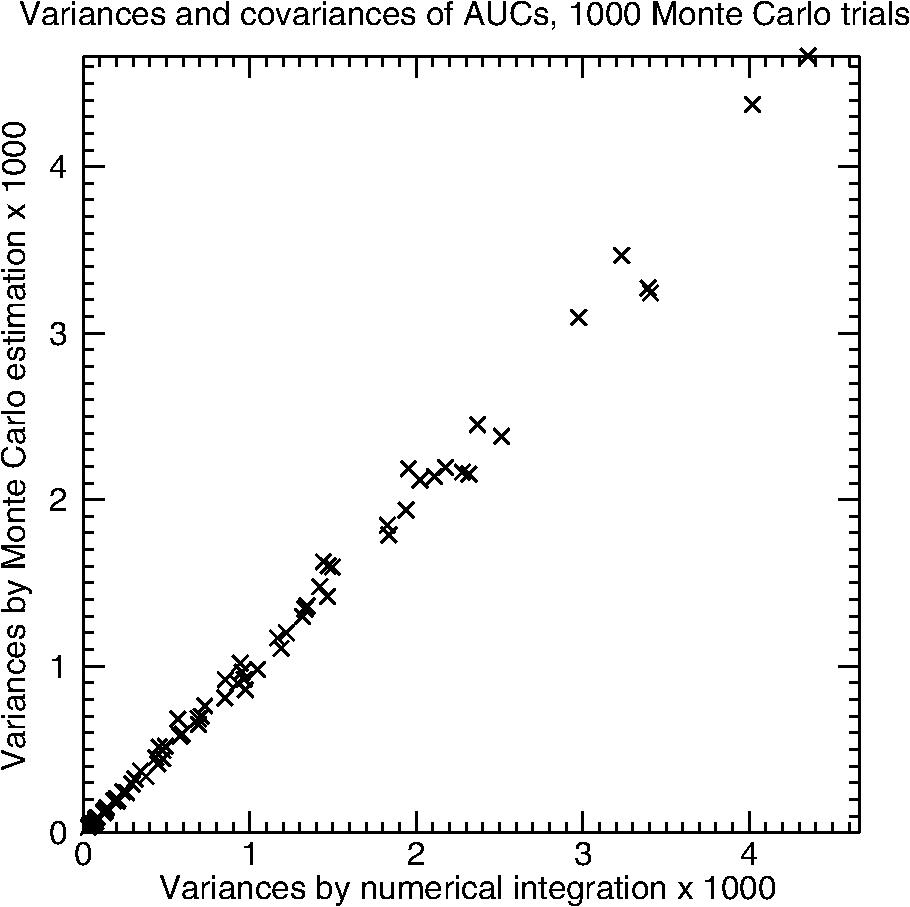

4. Conclusions

In this paper, we generalized the R&M model by allowing all of its variance components to depend on both modality and truth state. This will allow investigators to model and simulate MRMC ROC studies that better fit their data. Additionally, we presented and validated equations for computing the population variances and covariances for empirical AUC estimates computed from data simulated from the generalized R&M model. These equations show the core relationships between the ROC data and the reader-averaged AUCs. These equations and relationships should help investigators to validate new MRMC variance and covariance estimation methods, explore novel study designs, size future trials, and model MRMC ROC data.

For the interested investigator, the first author has made available a stand-alone Java application called iRoeMetz. iRoeMetz and its source code can be found in Ref. 35. iRoeMetz can simulate ROC studies according to the generalized R&M model and numerically calculate the expected moments and variances found in this paper. Additionally, all the original R&M simulation configurations and those used in this paper can be downloaded and tested.

Future work is needed in this area, investigating real data sets and calibrating the different possible R&M models of decision scores to be consistent with real data estimates of AUC variance components. To cover the full range, datasets that study different anatomical locations and diseases, and different imaging modalities (with and without computer aids as appropriate) are needed. The results of such future work would provide investigators with more information and examples to help them calibrate the R&M model (or any other model) to their situation so that they can appropriately size future reader studies. We are collecting datasets for this work for public sharing toward this goal; we welcome any and all contributions.

There are other interesting future efforts that could support the need mentioned above. One direction of study could link the success moments at the core of the work here to the parameters of the Obuchowski and Rockette³⁰ model for AUC observations. Another direction of study could be to uncover the inverse mapping: given the parameters of the Obuchowski and Rockette model for AUC observations, solve for the variance components of the ROC ratings that are consistent with them. It is not currently known whether the solution is unique or if it can be treated efficiently and effectively.

Appendices

Appendix A

In this appendix, we derive one of the product moments, ${[{\underset{̲}{M}}_{AB}]}_{5}$ , that enters into the computation of the covariance between ${\hat{AUC}}_{A}$ and ${\hat{AUC}}_{B}$ via Eq. (13). Adapting the results to the other moments that are required for computing the variance of ${\hat{AUC}}_{A}$ and the variance of ${\hat{AUC}}_{B}$ is straightforward.

Although the generalized R&M model has many parameters and the variances and the covariance of the reader-averaged AUCs are fairly complex, all of the success moments are derived the same way and the results have a common form. The derivations follow a common outline. The results are straightforward 1-D integrals involving the normal distribution that can be calculated using basic numerical integration methods. We illustrate the derivation for ${[{\underset{̲}{M}}_{AB}]}_{5}$ .

Here is the derivation outline:

1. Identify the random effects that are common to the two success observations. These will be the effects corresponding to shared subscripts.
2. Write the moment as the expected value of the product of two conditional expected values, one for each success observation. Each conditional expected value assumes that the random effects found in Step 1 are fixed.
3. Recognize that each conditional expected value equals a probability that can be expressed in the form $Φ (Z)$ , where $Z$ is a normal random variable equal to a difference in ROC ratings with the random effects found in Step 1 temporarily fixed.
4. Integrate over the random variables that were initially fixed in Step 1. This is a 1-D integral of the product of two normal cumulative distribution functions and one normal probability distribution function.

Step 1: The fifth product moment is

Eq. (18)

{[{\underset{̲}{M}}_{AB}]}_{5} = E (s_{A j k k^{'}} s_{B j^{'} k k^{'}}) = E [s (X_{A j k^{'} 1} - X_{A j k 0}) s (X_{B j^{'} k^{'} 1} - X_{B j^{'} k 0})] .

The random effects that are common to both success functions are the ones that do not depend on reader or modality:

{[C α]}_{k^{'} 1}, {[C α]}_{k 0}

. Note that these random effects are the effects corresponding to shared subscripts. This can be seen if we write out the differences in ROC ratings in terms of the constituent random effects.

Step 2: Here, we first write the moment as the expected value of a conditional expected value, where the random effects found in Step 1 are fixed; namely,

Eq. (19)

{[{\underset{̲}{M}}_{AB}]}_{5} = E [E (s_{A j k k^{'}} s_{B j^{'} k k^{'}} | {[C α]}_{k^{'} 1}, {[C α]}_{k 0})]

With the common random effects fixed,

s_{A j k k^{'}}

is independent of

s_{B j^{'} k k^{'}}

. Therefore, we can factor the conditional expected value to obtain

Eq. (20)

{[{\underset{̲}{M}}_{AB}]}_{5} = E [E (s_{A j k k^{'}} | {[C α]}_{k^{'} 1}, {[C α]}_{k 0}) E (s_{B j^{'} k k^{'}} | {[C α]}_{k^{'} 1}, {[C α]}_{k 0})] .

Step 3: In the expected value concerning modality A, the argument of the success function is a normal random variable $Z$ with mean and conditional variance given by

Eq. (21)

μ_{Z} = Δ_{A} + {[C α]}_{k^{'} 1} - {[C α]}_{k 0},

Eq. (22)

σ_{Z}^{2} = σ_{R 0}^{2} + σ_{R C 0}^{2} + σ_{R 1}^{2} + σ_{R C 1}^{2} + σ_{A R 0}^{2} + σ_{A C 0}^{2} + σ_{A R C 0}^{2} + σ_{A R 1}^{2} + σ_{A C 1}^{2} + σ_{A R C 1}^{2} .

Using the definitions given in Eq. (4) and Table 3, we see that

σ_{Z}^{2} = σ_{A}^{2} + σ_{Ω (5)}^{2}

. We have a similar result for the argument of the success function in the expected value concerning modality B. Since the argument to each conditional expected value is a normal random variable, we can write

Eq. (23)

{[{\underset{̲}{M}}_{AB}]}_{5} = E [Φ (\frac{Δ_{A} + {[C α]}_{k^{'} 1} - {[C α]}_{k 0}}{\sqrt{σ_{A}^{2} + σ_{Ω (5)}^{2}}}) Φ (\frac{Δ_{B} + {[C α]}_{k^{'} 1} - {[C α]}_{k 0}}{\sqrt{σ_{B}^{2} + σ_{Ω (5)}^{2}}})] .

Step 4: Last, we see that the only randomness that remains above is the difference ${[C α]}_{k^{'} 1} - {[C α]}_{k 0}$ . This difference is a normal random variable $Y = {[C α]}_{k^{'} 1} - {[C α]}_{k 0}$ with mean zero and variance $σ_{Ω}^{2} - σ_{Ω (5)}^{2} = σ_{C 0}^{2} + σ_{C 1}^{2}$ . After a change of variables, $X = Y / \sqrt{σ_{Ω}^{2} - σ_{Ω (5)}^{2}}$ we can effectively integrate over the random variables that were initially fixed, ${[C α]}_{k^{'} 1}, {[C α]}_{k 0}$ , with the following:

Eq. (24)

{[{\underset{̲}{M}}_{AB}]}_{5} = \int_{- \infty}^{\infty} Φ (\frac{Δ_{A} + x \sqrt{σ_{Ω}^{2} - σ_{Ω (5)}^{2}}}{\sqrt{σ_{A}^{2} + σ_{Ω (5)}^{2}}}) Φ (\frac{Δ_{B} + x \sqrt{σ_{Ω}^{2} - σ_{Ω (5)}^{2}}}{\sqrt{σ_{B}^{2} + σ_{Ω (5)}^{2}}}) ϕ (x) d x .

This last expression can be calculated using basic numerical integration methods. In our software, we simply sample the 1-D integral at 256 points on the interval (

- 10, 10

) and use the midpoint rule (rectangle rule).

Appendix B

Here, we document the simulation configurations used in this paper. We start by defining original R&M variance components. We then map them to generalized R&M variance components (Table 1). Finally, we perturb them to get variance structures that are different across modality and truth state.

The simulation configurations in this paper explore the following settings in a factorial fashion for 5 readers, 50 nondiseased cases, and 50 diseased cases:

• Two levels of between- and within-reader data correlation:
$\begin{matrix} High ρ_{BR} : & σ_{C}^{2} = 0.3 & σ_{τ C}^{2} = 0.3 & σ_{R C}^{2} = 0.2 & σ_{τ R C}^{2} = 0.2 \\ Low ρ_{BR} : & σ_{C}^{2} = 0.1 & σ_{τ C}^{2} = 0.1 & σ_{R C}^{2} = 0.2 & σ_{τ R C}^{2} = 0.6 \end{matrix}$
• Four levels of reader variability: $σ_{R}^{2} = σ_{τ R}^{2} = 0.0055$ , 0.011, 0.030, and 0.056.
• Three levels of performance: $Δ_{A} = Δ_{B} = α_{1} = 0.75$ , 1.50, and 2.5.

Let us consider the simulation with the high between- and within-reader data correlation and the lowest reader variability. After mapping and perturbing, the generalized R&M variance components are

\begin{matrix} σ_{R 0}^{2} = 0.0055, & σ_{C 0}^{2} = 0.3, & σ_{R C 0}^{2} = 0.2, & σ_{R 1}^{2} = 0.00550, & σ_{C 1}^{2} = 0.30, & σ_{R C 1}^{2} = 0.2, \\ σ_{A R 0}^{2} = 0.0055, & σ_{A C 0}^{2} = 0.3, & σ_{A R C 0}^{2} = 0.2, & σ_{A R 1}^{2} = 0.00275, & σ_{A C 1}^{2} = 0.15, & σ_{A R C 1}^{2} = 0.1, \\ σ_{B R 0}^{2} = 0.0055, & σ_{B C 0}^{2} = 0.3, & σ_{B R C 0}^{2} = 0.2, & σ_{B R 1}^{2} = 0.01100, & σ_{B C 1}^{2} = 0.60, & σ_{B R C 1}^{2} = 0.4 . \end{matrix}

This variance structure used with the lowest level of performance $(Δ_{A} = Δ_{B} = α_{1} = 0.75)$ leads to the following expectations of performance and uncertainty for 5 readers, 50 nondiseased cases, and 50 diseased cases:

\begin{matrix} {AUC}_{A} = 0.714, & \sqrt{var ({\hat{AUC}}_{A})} = 0.044, \\ {AUC}_{B} = 0.681, & \sqrt{var ({\hat{AUC}}_{B})} = 0.035, \\ {AUC}_{A} - {AUC}_{B} = 0.032, & \sqrt{var ({\hat{AUC}}_{A} - {\hat{AUC}}_{B})} = 0.047 . \end{matrix}

Acknowledgments

This research was partially supported by the National Institute of Biomedical Imaging and Bioengineering of the National Institutes of Health under Award Number R01EB013667. The content is solely the responsibility of the authors and does not necessarily represent the offical views of the National Institutes of Health, the Department of Veterans Affairs, or the United States government.

References

1.

B. D. Gallas et al., “Evaluating imaging and computer-aided detection and diagnosis devices at the FDA,” Acad. Radiol., 19 463 –477 (2012). http://dx.doi.org/10.1016/j.acra.2011.12.016 1076-6332 Google Scholar

2.

C. A. Roe and C. E. Metz, “Dorfman-Berbaum-Metz method for statistical analysis ofmultireader, multimodality receiver operating characteristic (ROC) data: validation with computer simulation,” Acad. Radiol., 4 (4), 298 –303 (1997). http://dx.doi.org/10.1016/S1076-6332(97)80032-3 1076-6332 Google Scholar

3.

D. D. Dorfman, K. S. Berbaum and C. E. Metz, “Receiver operating characteristic rating analysis: generalization to the population of readers and patients with the jackknife method,” Invest. Radiol., 27 (9), 723 –731 (1992). http://dx.doi.org/10.1097/00004424-199209000-00015 INVRAV 0020-9996 Google Scholar

4.

S. V. Beiden, R. F. Wagner and G. Campbell, “Components-of-variance models and multiple-bootstrap experiments: an alternative method for random-effects, receiver operating characteristic analysis,” Acad. Radiol., 7 (5), 341 –349 (2000). http://dx.doi.org/10.1016/S1076-6332(00)80008-2 1076-6332 Google Scholar

5.

S. V. Beiden et al., “Analysis of uncertainties in estimates of components of variance in multivariate ROC analysis,” Acad. Radiol., 8 (7), 616 –622 (2001). http://dx.doi.org/10.1016/S1076-6332(03)80686-4 1076-6332 Google Scholar

6.

X. Song and X.-H. Zhou, “A marginal model approach for analysis of multi-reader multi-test receiver operating characteristic (ROC) data,” Biostatistics, 6 (2), 303 –312 (2005). http://dx.doi.org/10.1093/biostatistics/kxi011 1465-4644 Google Scholar

7.

S. L. Hillis and K. S. Berbaum, “Monte Carlo validation of the Dorfman-Berbaum-Metz method using normalized pseudovalues and less data-based model simplification,” Acad. Radiol., 12 (12), 1534 –1541 (2005). http://dx.doi.org/10.1016/j.acra.2005.07.012 1076-6332 Google Scholar

8.

S. L. Hillis, “A comparison of denominator degrees of freedom methods for multiple observer ROC analysis,” Stat. Med., 26 (3), 596 –619 (2007). http://dx.doi.org/10.1002/(ISSN)1097-0258 SMEDDA 1097-0258 Google Scholar

9.

S. L. Hillis, K. S. Berbaum and C. E. Metz, “Recent developments in the Dorfman-Berbaum-Metz procedure for multireader ROC study analysis,” Acad. Radiol., 15 (5), 647 –661 (2008). http://dx.doi.org/10.1016/j.acra.2007.12.015 1076-6332 Google Scholar

10.

A. Skaron, K. Li and X.-H. Zhou, “Statistical methods for MRMC ROC studies,” Acad. Radiol., 19 (12), 1499 –1507 (2012). http://dx.doi.org/10.1016/j.acra.2012.09.005 1076-6332 Google Scholar

11.

D. P. Chakraborty, “Prediction accuracy of a sample-size estimation method for ROC studies,” Acad. Radiol., 17 (5), 628 –638 (2010). http://dx.doi.org/10.1016/j.acra.2010.01.007 1076-6332 Google Scholar

12.

S. L. Hillis, N. A. Obuchowski and K. S. Berbaum, “Power estimation for multireader ROC methods an updated and unified approach,” Acad. Radiol., 18 (2), 129 –142 (2011). http://dx.doi.org/10.1016/j.acra.2010.09.007 1076-6332 Google Scholar

13.

D. D. Dorfman et al., “Monte Carlo validation of a multireader method for receiver operating characteristic discrete rating data: factorial experimental design,” Acad. Radiol., 5 (9), 591 –602 (1998). http://dx.doi.org/10.1016/S1076-6332(98)80294-8 1076-6332 Google Scholar

14.

R. F. Wagner, S. V. Beiden and C. E. Metz, “Continuous versus categorical data for ROC analysis: some quantitative considerations,” Acad. Radiol., 8 (4), 328 –334 (2001). http://dx.doi.org/10.1016/S1076-6332(03)80502-0 1076-6332 Google Scholar

15.

N. Obuchowski, B. D. Gallas and S. L. Hillis, “Multi-reader ROC studies with split-plot designs: a comparison of statistical methods,” Acad. Radiol., 19 (12), 1508 –1517 (2012). http://dx.doi.org/10.1016/j.acra.2012.09.012 1076-6332 Google Scholar

16.

B. D. Gallas, G. A. Pennello and K. J. Myers, “Multireader multicase variance analysis for binary data,” J. Opt. Soc. Am. A, Spec. Issue on Image Qual., 24 (12), B70 –B80 (2007). http://dx.doi.org/10.1364/JOSAA.24.000B70 JOAOD6 0740-3232 Google Scholar

17.

W. Chen et al., “A general framework for MRMC reader studies with binary assessments: simulation for validation and sizing,” JMI, (2014). Google Scholar

18.

C. K. Abbey, F. W. Samuelson and B. D. Gallas, “Statistical power considerations for a utility endpoint in observer performance studies,” Acad. Radiol., 20 (7), 798 –806 (2013). http://dx.doi.org/10.1016/j.acra.2013.02.008 1076-6332 Google Scholar

19.

S. L. Hillis, “Simulation of unequal-variance binormal multireader ROC decision data: an extension of the Roe and Metz simulation model,” Acad. Radiol., 19 (12), 1518 –1528 (2012). http://dx.doi.org/10.1016/j.acra.2012.09.011 1076-6332 Google Scholar

20.

S. V. Beiden et al., “Components-of-variance models for random-effects ROC analysis: the case of unequal variance structures across modalities,” Acad. Radiol., 8 (7), 605 –615 (2001). http://dx.doi.org/10.1016/S1076-6332(03)80685-2 1076-6332 Google Scholar

21.

J. Swets, W. P. Tanner and T. G. Birdsall, “Decision processes in perception,” Psychol. Rev., 68 (5), 301 –340 (1961). http://dx.doi.org/10.1037/h0040547 PSRVAX 0033-295X Google Scholar

22.

D. M. Green and J. A. Swets, Signal Detection Theory and Psychophysics, Wiley, New York (1966). Google Scholar

23.

H. P. Chan et al., “Digital mammography: observer performance study of the effects of pixel size on the characterization of malignant and benign microcalcifications,” Acad. Radiol., 8 (6), 454 –466 (2001). http://dx.doi.org/10.1016/S1076-6332(03)80616-5 1076-6332 Google Scholar

24.

B. Sahiner et al., “Multi-modality CADx: ROC study of the effect on radiologists’ accuracy in characterizing breast masses on mammograms and 3D ultrasound images,” Acad. Radiol., 16 (7), 810 –818 (2009). http://dx.doi.org/10.1016/j.acra.2009.01.011 1076-6332 Google Scholar

25.

E. A. Rafferty et al., “Assessing radiologist performance using combined digital mammography and breast tomosynthesis compared with digital mammography alone: results of a multicenter, multireader trial,” Radiology, 266 (1), 104 –113 (2013). http://dx.doi.org/10.1148/radiol.12120674 RADLAX 0033-8419 Google Scholar

26.

F. W. Samuelson and X. He, “Comparison of semiparametric receiver operating characteristic models on observer data,” J. Med. Imag., 1 (3), 031004 (2014). http://dx.doi.org/10.1117/1.JMI.1.3.031004 Google Scholar

27.

D. D. Dorfman and K. S. Berbaum, “A contaminated binormal model for ROC data: Part II. A formal model,” Acad. Radiol., 7 (6), 427 –437 (2000). http://dx.doi.org/10.1016/S1076-6332(00)80383-9 1076-6332 Google Scholar

28.

C. E. Metz and X. Pan, “Proper’ binormal ROC curves: theory and maximum-likelihood estimation,” J. Math. Psychol., 43 (1), 1 –33 (1999). http://dx.doi.org/10.1006/jmps.1998.1218 JMTPAJ 0022-2496 Google Scholar

29.

L. L. Pesce and C. E. Metz, “Reliable and computationally efficient maximum-likelihood estimation of “proper” binormal ROC curves,” Acad. Radiol., 14 (7), 814 –829 (2007). http://dx.doi.org/10.1016/j.acra.2007.03.012 1076-6332 Google Scholar

30.

N. A. Obuchowski and H. E. Rockette, “Hypothesis testing of diagnostic accuracy for multiple readers and multiple tests: an ANOVA approach with dependent observations,” Commun. Stat. B-Simul., 24 (2), 285 –308 (1995). http://dx.doi.org/10.1080/03610919508813243 0361-0918 Google Scholar

31.

R. E. Kirk, Experimental Design: Procedures for the Behavioral Sciences, 3rd ed.Wadsworth Publishing, Belmont, CA (1994). Google Scholar

32.

E. R. DeLong, D. M. Delong and D. L. Clarke-Pearson, “Comparing the areas under two or more correlated receiver operating characteristic curves: a nonparametric approach,” Biometrics, 44 (3), 837 –845 (1988). http://dx.doi.org/10.2307/2531595 BIOMB6 0006-341X Google Scholar

33.

B. D. Gallas et al., “A framework for random-effects ROC analysis: biases with the bootstrap and other variance estimators,” Commun. Stat. A-Theory, 38 (15), 2586 –2603 (2009). http://dx.doi.org/10.1080/03610920802610084 0361-0926 Google Scholar

34.

C. E. Metz, P. L. Wang and K. B. Kronman, “A new approach for testing the significance of differences between ROC curves measured from correlated data,” Information Processing in Medical Imaging VIII, 432 –445 Springer, Netherlands (1984). Google Scholar

35.

B. D. Gallas, “iROEMETZ v1.2: Application for Simulating MRMC Reader Studies,” (2014) code.google.com/p/imrmc/wiki/iRoeMetzGuide August ). 2014). Google Scholar

Biography

Brandon D. Gallas provides mathematical, statistical, and modeling expertise to the evaluation of medical imaging devices at the FDA. His main areas of contribution are in the design and statistical analysis of reader studies, image quality, computer-aided diagnosis, and imaging physics. Before working at the FDA, he was in Dr. Harrison Barrett’s research group at the University of Arizona, earning his PhD from the Graduate Interdisciplinary Program in Applied Mathematics.

Stephen L. Hillis is a research professor in the Departments of Radiology and Biostatistics at the University of Iowa, and Senior Statistician for the Iowa City VA Healthcare System. He earned his PhD in statistics from the University of Iowa in 1987 and is the author of 85 peer-reviewed articles. Since 1998 his research has focused on methodology for analyzing diagnostic radiological imaging studies.

CC BY: © The Authors. Published by SPIE under a Creative Commons Attribution 4.0 Unported License. Distribution or reproduction of this work in whole or in part requires full attribution of the original publication, including its DOI.

Citation Download Citation

Brandon D. Gallas and Stephen L. Hillis "Generalized Roe and Metz receiver operating characteristic model: analytic link between simulated decision scores and empirical AUC variances and covariances," Journal of Medical Imaging 1(3), 031006 (25 September 2014). https://doi.org/10.1117/1.JMI.1.3.031006

Published: 25 September 2014

Access the abstract

JOURNAL ARTICLE
9 PAGES

DOWNLOAD PAPER SAVE TO MY LIBRARY

GET CITATION

CITATIONS

Cited by 17 scholarly publications.

Explore citations on Lens.org

KEYWORDS

Data modeling

Monte Carlo methods

Receivers

Computer simulations

Performance modeling

Numerical integration

Statistical analysis

1.

Introduction

2.

Methods

2.1.

Generalized Roe and Metz Model

Eq. (1)

2.1.1.

Updated notation

Eq. (2)

2.1.2.

Allow variances to depend on modality and truth

Eq. (3)

Eq. (4)

Eq. (5)

Table 1

2.2.

Expected AUCs

Eq. (6)

Eq. (7)

Eq. (8)

Eq. (9)

2.3.

Variances and Covariances

Eq. (10)

2.3.1.

Variance

Eq. (11)

Table 2

Table 3

Eq. (12)

2.3.2.

Covariance

Eq. (13)

Eq. (14)

Eq. (15)

2.4.

Design of Simulation Studies

Eq. (16)

Eq. (17)

3.

Results

Fig. 1

4.

Conclusions

Appendices

Appendix A

Eq. (18)

Eq. (19)

Eq. (20)

Eq. (21)

Eq. (22)

Eq. (23)

Eq. (24)

Appendix B

Acknowledgments

References

Biography

Show All Keywords

Keywords/Phrases

Search In:

Publication Years